Sample success is defined as the percentage of samples which amplify
a specific percentage of loci given the allele detection coverage
threshold or number of paired reads that support the allele or ASV in a
sample. Here we are going to show 6 different coverage thresholds: 1, 5,
10, 20, 50, and 100 paired reads.
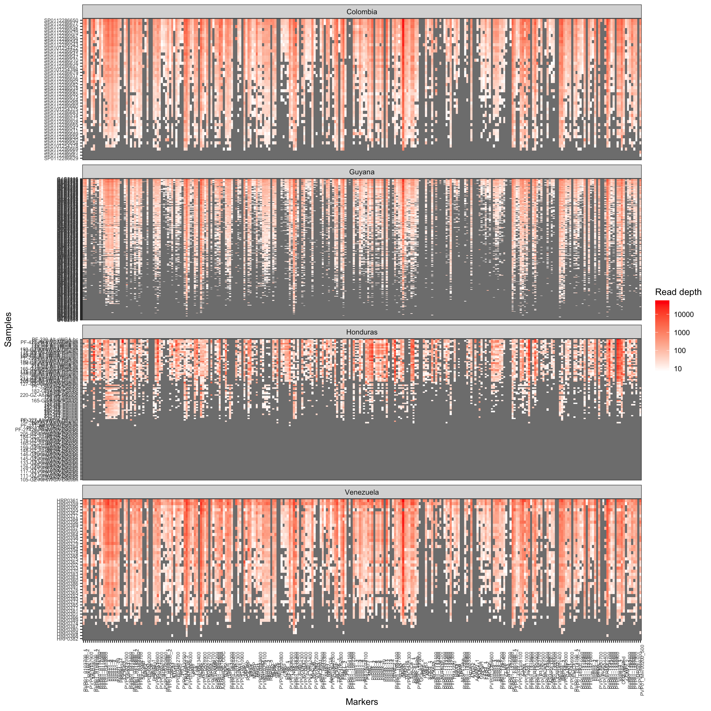
Overall sequencing yield
Measure the read coverage by using the function
get_ReadDepth_coverage:
ReadDepth_coverage = get_ReadDepth_coverage(ampseq_object_abd1, variable = NULL)
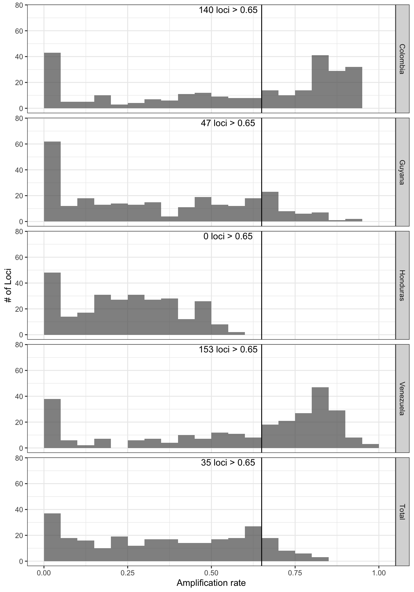
For each sample, calculates how many loci has a read depth equals or
greater than 1, 5, 10, 20, 50, or 100:
sample_performance = ReadDepth_coverage$plot_read_depth_heatmap$data %>%
    mutate(Read_depth = case_when(
      is.na(Read_depth) ~ 0,
      !is.na(Read_depth) ~ Read_depth
    )) %>%
    summarise(amplified_amplicons1 = sum(Read_depth >= 1)/nrow(ampseq_object_abd1@markers),
              amplified_amplicons5 = sum(Read_depth >= 5)/nrow(ampseq_object_abd1@markers),
              amplified_amplicons10 = sum(Read_depth >= 10)/nrow(ampseq_object_abd1@markers),
              amplified_amplicons20 = sum(Read_depth >= 20)/nrow(ampseq_object_abd1@markers),
              amplified_amplicons50 = sum(Read_depth >= 50)/nrow(ampseq_object_abd1@markers),
              amplified_amplicons100 = sum(Read_depth >= 100)/nrow(ampseq_object_abd1@markers),
              .by = Sample_id) %>%
    pivot_longer(cols = starts_with('amplified_amplicons'), values_to = 'AmpRate', names_to = 'Threshold') %>%
    mutate(Threshold = as.integer(gsub('amplified_amplicons', '', Threshold)))
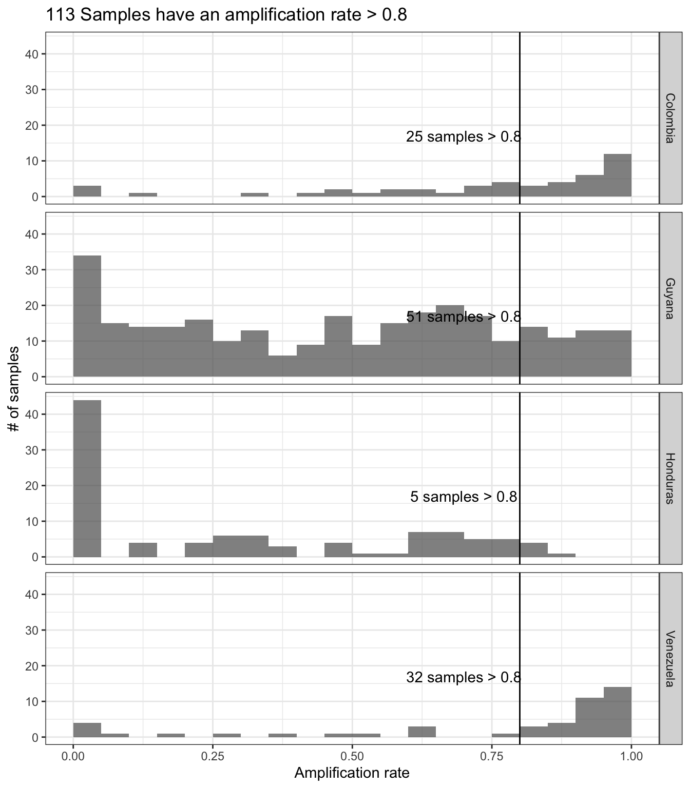
Generate a plot showing the percentage of loci (amplicon or marker)
which contains alleles that pass the thresholds in the x-axis, and the
percentage of samples which amplify a specific percentage of loci given
the allele detection thresholds in the y-axis. Include a vertical line
that indicates samples that has amplify at least 50% of the loci with
the especific read depth coverage.
plot_precentage_of_samples_over_min_abd = sample_performance %>%
    summarise(AmpRate5 = round(100*sum(AmpRate >= .05)/n(), 1),
              AmpRate10 = round(100*sum(AmpRate >= .10)/n(), 1),
              AmpRate15 = round(100*sum(AmpRate >= .15)/n(), 1),
              AmpRate20 = round(100*sum(AmpRate >= .20)/n(), 1),
              AmpRate25 = round(100*sum(AmpRate >= .25)/n(), 1),
              AmpRate30 = round(100*sum(AmpRate >= .30)/n(), 1),
              AmpRate35 = round(100*sum(AmpRate >= .35)/n(), 1),
              AmpRate40 = round(100*sum(AmpRate >= .40)/n(), 1),
              AmpRate45 = round(100*sum(AmpRate >= .45)/n(), 1),
              AmpRate50 = round(100*sum(AmpRate >= .50)/n(), 1),
              AmpRate55 = round(100*sum(AmpRate >= .55)/n(), 1),
              AmpRate60 = round(100*sum(AmpRate >= .60)/n(), 1),
              AmpRate65 = round(100*sum(AmpRate >= .65)/n(), 1),
              AmpRate70 = round(100*sum(AmpRate >= .70)/n(), 1),
              AmpRate75 = round(100*sum(AmpRate >= .75)/n(), 1),
              AmpRate80 = round(100*sum(AmpRate >= .80)/n(), 1),
              AmpRate85 = round(100*sum(AmpRate >= .85)/n(), 1),
              AmpRate90 = round(100*sum(AmpRate >= .90)/n(), 1),
              AmpRate95 = round(100*sum(AmpRate >= .95)/n(), 1),
              AmpRate100 = round(100*sum(AmpRate >= 1)/n(), 1),
              .by = c(Threshold)
    ) %>%
    pivot_longer(cols = paste0('AmpRate', seq(5, 100, 5)),
                 values_to = 'Percentage',
                 names_to = 'AmpRate') %>%
    mutate(AmpRate = as.numeric(gsub('AmpRate','', AmpRate)))%>%
    ggplot(aes(x = AmpRate, y = Percentage, color = as.factor(Threshold), group = as.factor(Threshold))) +
    geom_line() +
    geom_vline(xintercept = 50, linetype = 2) +
    theme_bw() +
    labs(x = '% of amplified loci (amplification rate)', y = '% of Samples', color = 'Min Coverage')
plot_precentage_of_samples_over_min_abd
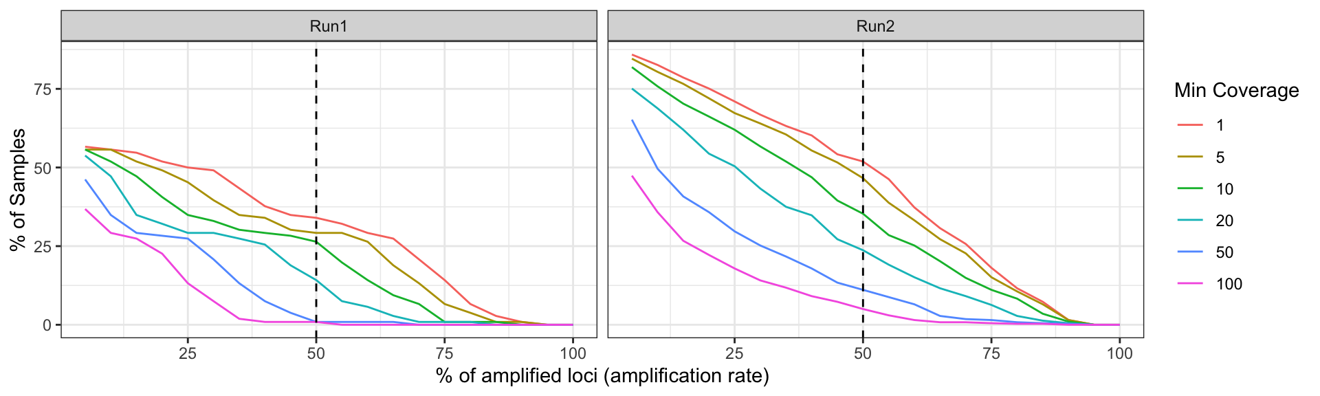
Let’s check the performance by sequencing run
ReadDepth_coverage = get_ReadDepth_coverage(ampseq_object_abd1, variable = 'Run')

sample_performance = ReadDepth_coverage$plot_read_depth_heatmap$data %>%
    mutate(Read_depth = case_when(
      is.na(Read_depth) ~ 0,
      !is.na(Read_depth) ~ Read_depth
    )) %>%
    summarise(amplified_amplicons1 = sum(Read_depth >= 1)/nrow(ampseq_object_abd1@markers),
              amplified_amplicons5 = sum(Read_depth >= 5)/nrow(ampseq_object_abd1@markers),
              amplified_amplicons10 = sum(Read_depth >= 10)/nrow(ampseq_object_abd1@markers),
              amplified_amplicons20 = sum(Read_depth >= 20)/nrow(ampseq_object_abd1@markers),
              amplified_amplicons50 = sum(Read_depth >= 50)/nrow(ampseq_object_abd1@markers),
              amplified_amplicons100 = sum(Read_depth >= 100)/nrow(ampseq_object_abd1@markers),
              Run = unique(var),
              .by = Sample_id) %>%
    pivot_longer(cols = starts_with('amplified_amplicons'), values_to = 'AmpRate', names_to = 'Threshold') %>%
    mutate(Threshold = as.integer(gsub('amplified_amplicons', '', Threshold)))

plot_precentage_of_samples_over_min_abd_byRun = sample_performance %>%
    summarise(AmpRate5 = round(100*sum(AmpRate >= .05)/n(), 1),
              AmpRate10 = round(100*sum(AmpRate >= .10)/n(), 1),
              AmpRate15 = round(100*sum(AmpRate >= .15)/n(), 1),
              AmpRate20 = round(100*sum(AmpRate >= .20)/n(), 1),
              AmpRate25 = round(100*sum(AmpRate >= .25)/n(), 1),
              AmpRate30 = round(100*sum(AmpRate >= .30)/n(), 1),
              AmpRate35 = round(100*sum(AmpRate >= .35)/n(), 1),
              AmpRate40 = round(100*sum(AmpRate >= .40)/n(), 1),
              AmpRate45 = round(100*sum(AmpRate >= .45)/n(), 1),
              AmpRate50 = round(100*sum(AmpRate >= .50)/n(), 1),
              AmpRate55 = round(100*sum(AmpRate >= .55)/n(), 1),
              AmpRate60 = round(100*sum(AmpRate >= .60)/n(), 1),
              AmpRate65 = round(100*sum(AmpRate >= .65)/n(), 1),
              AmpRate70 = round(100*sum(AmpRate >= .70)/n(), 1),
              AmpRate75 = round(100*sum(AmpRate >= .75)/n(), 1),
              AmpRate80 = round(100*sum(AmpRate >= .80)/n(), 1),
              AmpRate85 = round(100*sum(AmpRate >= .85)/n(), 1),
              AmpRate90 = round(100*sum(AmpRate >= .90)/n(), 1),
              AmpRate95 = round(100*sum(AmpRate >= .95)/n(), 1),
              AmpRate100 = round(100*sum(AmpRate >= 1)/n(), 1),
              .by = c(Threshold, Run)
    ) %>%
    pivot_longer(cols = paste0('AmpRate', seq(5, 100, 5)),
                 values_to = 'Percentage',
                 names_to = 'AmpRate') %>%
    mutate(AmpRate = as.numeric(gsub('AmpRate','', AmpRate)))%>%
    ggplot(aes(x = AmpRate, y = Percentage, color = as.factor(Threshold), group = as.factor(Threshold))) +
    geom_line() +
    geom_vline(xintercept = 50, linetype = 2) +
    facet_wrap(Run~., ncol = 3)+
    theme_bw() +
    labs(x = '% of amplified loci (amplification rate)', y = '% of Samples', color = 'Min Coverage')
plot_precentage_of_samples_over_min_abd_byRun
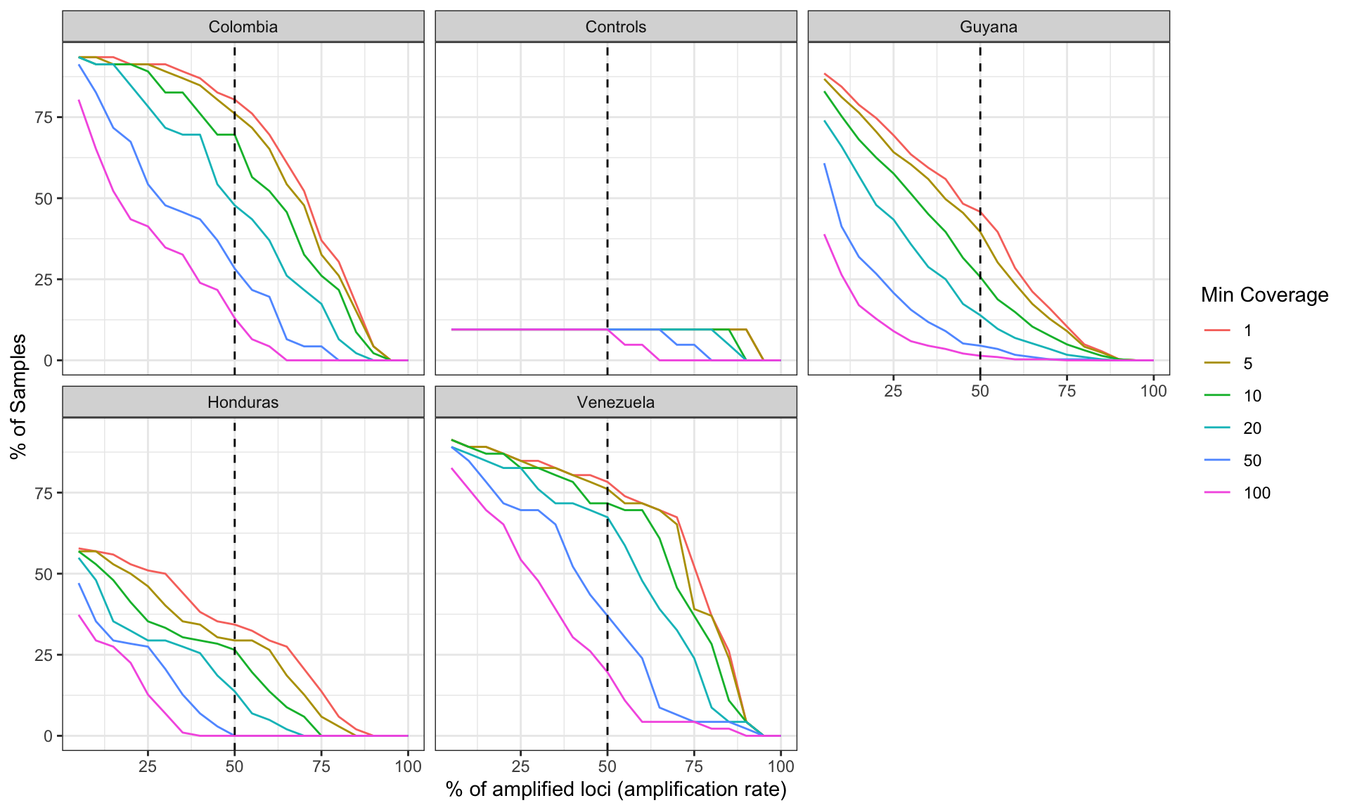
Let’s do it by Country
ReadDepth_coverage = get_ReadDepth_coverage(ampseq_object_abd1, variable = 'Country')

sample_performance = ReadDepth_coverage$plot_read_depth_heatmap$data %>%
      filter(!is.na(var))%>%
      mutate(Read_depth = case_when(
        is.na(Read_depth) ~ 0,
        !is.na(Read_depth) ~ Read_depth
      )) %>%
      summarise(amplified_amplicons1 = sum(Read_depth >= 1)/nrow(ampseq_object_abd1@markers),
                amplified_amplicons5 = sum(Read_depth >= 5)/nrow(ampseq_object_abd1@markers),
                amplified_amplicons10 = sum(Read_depth >= 10)/nrow(ampseq_object_abd1@markers),
                amplified_amplicons20 = sum(Read_depth >= 20)/nrow(ampseq_object_abd1@markers),
                amplified_amplicons50 = sum(Read_depth >= 50)/nrow(ampseq_object_abd1@markers),
                amplified_amplicons100 = sum(Read_depth >= 100)/nrow(ampseq_object_abd1@markers),
                Country = unique(var),
                .by = Sample_id) %>%
      pivot_longer(cols = starts_with('amplified_amplicons'), values_to = 'AmpRate', names_to = 'Threshold') %>%
      mutate(Threshold = as.integer(gsub('amplified_amplicons', '', Threshold)))

plot_precentage_of_samples_over_min_abd_byCountry = sample_performance %>%
      summarise(AmpRate5 = round(100*sum(AmpRate >= .05)/n(), 1),
                AmpRate10 = round(100*sum(AmpRate >= .10)/n(), 1),
                AmpRate15 = round(100*sum(AmpRate >= .15)/n(), 1),
                AmpRate20 = round(100*sum(AmpRate >= .20)/n(), 1),
                AmpRate25 = round(100*sum(AmpRate >= .25)/n(), 1),
                AmpRate30 = round(100*sum(AmpRate >= .30)/n(), 1),
                AmpRate35 = round(100*sum(AmpRate >= .35)/n(), 1),
                AmpRate40 = round(100*sum(AmpRate >= .40)/n(), 1),
                AmpRate45 = round(100*sum(AmpRate >= .45)/n(), 1),
                AmpRate50 = round(100*sum(AmpRate >= .50)/n(), 1),
                AmpRate55 = round(100*sum(AmpRate >= .55)/n(), 1),
                AmpRate60 = round(100*sum(AmpRate >= .60)/n(), 1),
                AmpRate65 = round(100*sum(AmpRate >= .65)/n(), 1),
                AmpRate70 = round(100*sum(AmpRate >= .70)/n(), 1),
                AmpRate75 = round(100*sum(AmpRate >= .75)/n(), 1),
                AmpRate80 = round(100*sum(AmpRate >= .80)/n(), 1),
                AmpRate85 = round(100*sum(AmpRate >= .85)/n(), 1),
                AmpRate90 = round(100*sum(AmpRate >= .90)/n(), 1),
                AmpRate95 = round(100*sum(AmpRate >= .95)/n(), 1),
                AmpRate100 = round(100*sum(AmpRate >= 1)/n(), 1),
                .by = c(Threshold, Country)
      ) %>%
      pivot_longer(cols = paste0('AmpRate', seq(5, 100, 5)),
                   values_to = 'Percentage',
                   names_to = 'AmpRate') %>%
      mutate(AmpRate = as.numeric(gsub('AmpRate','', AmpRate)))%>%
      ggplot(aes(x = AmpRate, y = Percentage, color = as.factor(Threshold), group = as.factor(Threshold))) +
      geom_line() +
      geom_vline(xintercept = 50, linetype = 2) +
      facet_wrap(Country~., ncol = 3)+
      theme_bw() +
      labs(x = '% of amplified loci (amplification rate)', y = '% of Samples', color = 'Min Coverage')
plot_precentage_of_samples_over_min_abd_byCountry