Genetic Relatedness (IBD) and Connectivity
Neafsey Lab
The genetic relatedness between individual parasite haplotypes and among parasite populations has several practical uses in the study of malaria. For example, relatedness information can help determine the geographic origin of imported infections, define the extent to which parasites are dispersing or are contained within landscapes, and identify whether specific strains are being selected for over time. Relatedness information is also very helpful in understanding longitudinal (within-individual) infection dynamics. In the case of P. vivax, for example, it can distinguish whether infection represents newly acquired parasites, recrudescence after treatment, or relapse from longer-lasting hypnozoite reservoirs. Relatedness information can also help resolve polyclonality signals, i.e., clarify the number of different haplotypes co-infecting individual patients.
Relatedness is defined as the probability that, at any locus in the genome, the alleles sampled from two different individuals are identical by descent (\(IBD\)). Genetic markers used for this purpose include SNPs, microsatellites, and (increasingly) amplicon micro-haplotypes (MHAP). Relatedness can be estimated using a Hidden Markov Model approach implemented in the R package paneljudge (see mathematical framework in AR Taylor et al. 2019). In this package, relatedness (\(r\)) is estimated as a function of the haplotype of the two sampled parasites (\(Y^{(i)}\) and \(Y^{(j)}\), where \(i\) and \(j\) denote two different sampled genotypes from the population), the frequency of the alleles in the population (\(f_t(g)\), where \(t\) denotes locus), the physical distance (\(d_t\), in base-pairs) between successively analyzed loci (\(t-1\) and \(t\)), the recombination rate (\(\rho\)), a switching rate of the Markov chain (\(k\)), and a constant genotyping error rate (\(\varepsilon\)).
Pairwise relatedness comparisons between categories
For this report all possible pairwise IBD comparisons between samples from different categories of Variable1 and Variable2 are computed, and the results are shown in the following table:
source('~/Documents/Github/intro_to_genomic_surveillance/docs/functions_and_libraries/amplseq_required_libraries.R')
source('~/Documents/Github/intro_to_genomic_surveillance/docs/functions_and_libraries/amplseq_functions.R')
#sourceCpp('~/Documents/Github/intro_to_genomic_surveillance/docs/functions_and_libraries/hmmloglikelihood.cpp')
Read the ampseq_object in csv format:
ampseq_object = read_ampseq(file = '~/Documents/Github/intro_to_genomic_surveillance/docs/data/Pfal_example/Pfal_ampseq_filtered',
                   format = 'csv')
Run the function pairwise_hmmIBD:
pairwise_relatedness_table = '~/Documents/Github/intro_to_genomic_surveillance/docs/data/Pfal_example/pairwise_relatedness.csv'

if(!file.exists(pairwise_relatedness_table)){
      pairwise_relatedness = NULL

      nChunks = 500

      for(w in nChunks){
        start = Sys.time()
        pairwise_relatedness = rbind(pairwise_relatedness,
                                     pairwise_hmmIBD(ampseq_object, parallel = TRUE, w = w, n = nChunks))
        time_diff = Sys.time() - start

        print(paste0('step ', w, ' done in ', time_diff, ' secs'))

      }

      write.csv(pairwise_relatedness,
                '~/Documents/Github/intro_to_genomic_surveillance/docs/data/Pfal_example/pairwise_relatedness.csv',
                quote = FALSE,
                row.names = FALSE)

    }else{

      pairwise_relatedness = read.csv(pairwise_relatedness_table)

    }
Plot the distribution of relatedness between sites using the function
plot_relatedness_distribution
plot_relatedness_distribution_between = plot_relatedness_distribution(
      pairwise_relatedness = pairwise_relatedness,
      metadata = ampseq_object@metadata,
      Population = 'Subnational_level2',
      fill_color = rep('gray50', length(unique(ampseq_object@metadata[['Subnational_level2']]))*(length(unique(ampseq_object@metadata[['Subnational_level2']]))-1)/2),
      type_pop_comparison = 'between',
      ncol = 3,
      pop_levels = NULL
)View(plot_relatedness_distribution_between$relatedness)The distribution of pairwise genetic relatedness values is presented using histograms as follows:
plot_relatedness_distribution_between$plot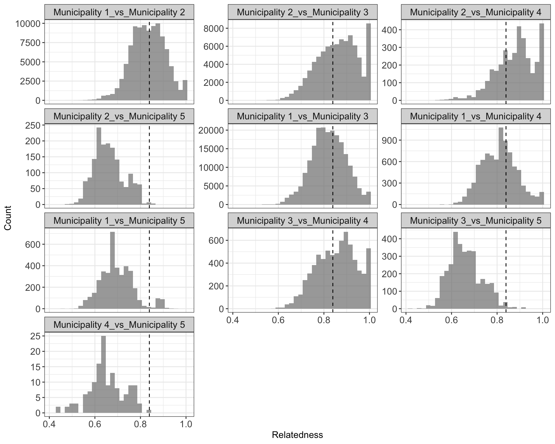
Figure 1: Pairwise IBD distribution between categories of Variable1 (panels). The x-axis shows genetic relatedness values, ranging from 0 (unrelated) to 1 (clonal). The y-axis shows the number of pairwise comparisons corresponding to each of these relatedness values. The dotted vertical line represents the median genetic relatedness in the total dataset (including both within and between-population comparisons).
Fraction of highly related comparisons between categories of Variable1
Based on the defined threshold (0.99), highly related pairwise comparisons between categories in Subnational_level2 are counted and proportions with their 95% CI (Fisher exact test) are calculated.
plot_frac_highly_related_between = plot_frac_highly_related(
      pairwise_relatedness = pairwise_relatedness,
      metadata = ampseq_object@metadata,
      Population = 'Subnational_level2',
      fill_color = rep('gray50', length(unique(ampseq_object@metadata[['Subnational_level2']]))*(length(unique(ampseq_object@metadata[['Subnational_level2']]))-1)/2),
      threshold = 0.99,
      type_pop_comparison = 'between',
      pop_levels = NULL)
These values are presented in the following table and in Figure 2:
View(plot_frac_highly_related_between$highly_related_table)plot_frac_highly_related_between$plot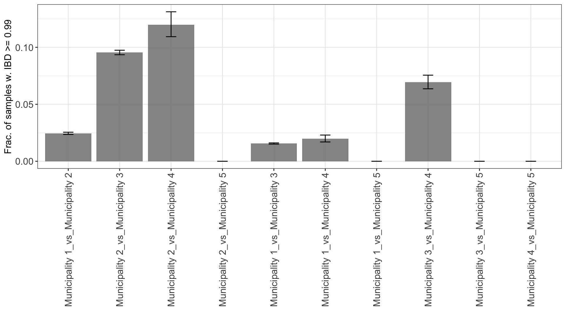
Figure 2: Fraction of highly related pairwise comparisons (IBD >= ibd_thres) between categories of Variable1 (x-axis). 95% confidence intervals are computed using a Fisher exact test.
Fraction of highly related comparisons between categories of Variable1 over Variable2
Highly related pairwise comparisons between categories in Subnational_level2 and Quarter_of_Collection are also counted and proportions with their 95% CI (Fisher exact test) are calculated.
plot_frac_highly_related_overtime_between = plot_frac_highly_related_over_time(
        pairwise_relatedness = pairwise_relatedness,
        metadata = ampseq_object@metadata,
        Population = c('Subnational_level2', 'Quarter_of_Collection'),
        fill_color = rep('gray50', length(unique(ampseq_object@metadata[['Subnational_level2']]))*(length(unique(ampseq_object@metadata[['Subnational_level2']]))-1)/2),
        threshold = 0.99,
        type_pop_comparison = 'between',
        ncol = 3,
        pop_levels = NULL)
These values are presented in the following table and in Figures 3-4:
View(plot_frac_highly_related_overtime_between$frac_highly_related)plot_frac_highly_related_overtime_between$plot_IBD_correlation_matrix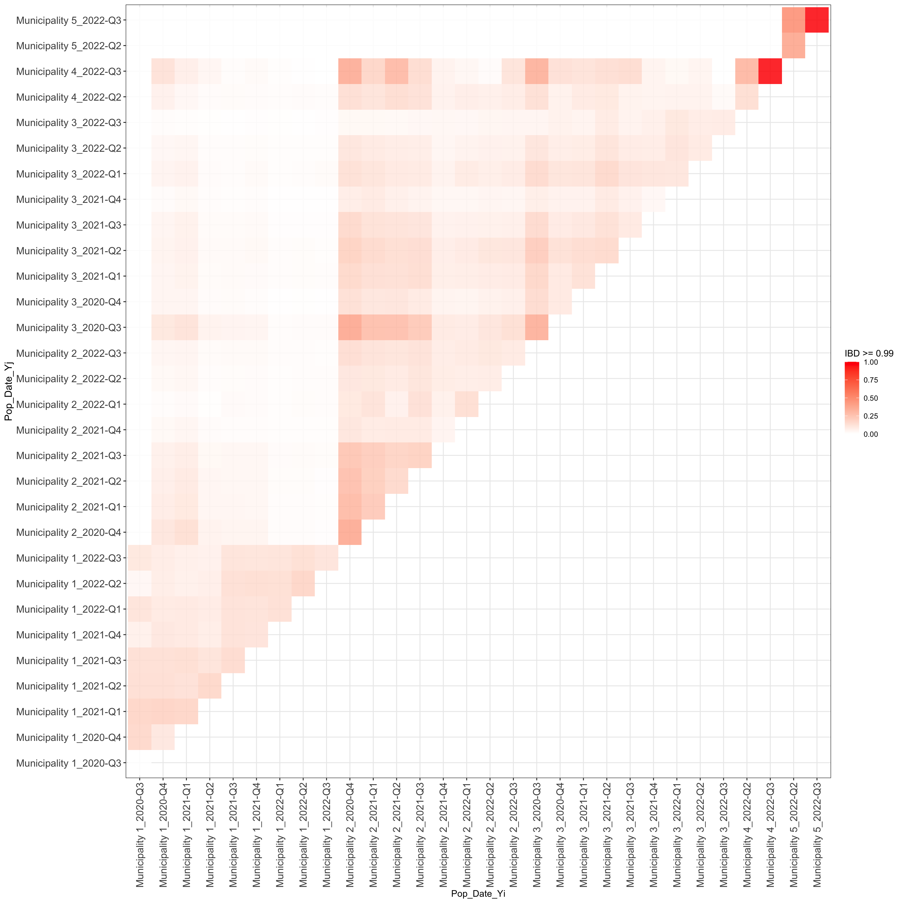
Figure 3: Heatmap matrix of the fraction of highly related pairwise comparisons (IBD >= ibd_thres) between categories of Variable1 and Variable2. The color scale indicates the fraction of highly related samples (increasing with higher intensities of red). The diagonal in the matrix represents pairwise comparisons within categories.
plot_frac_highly_related_overtime_between$plot_frac_highly_related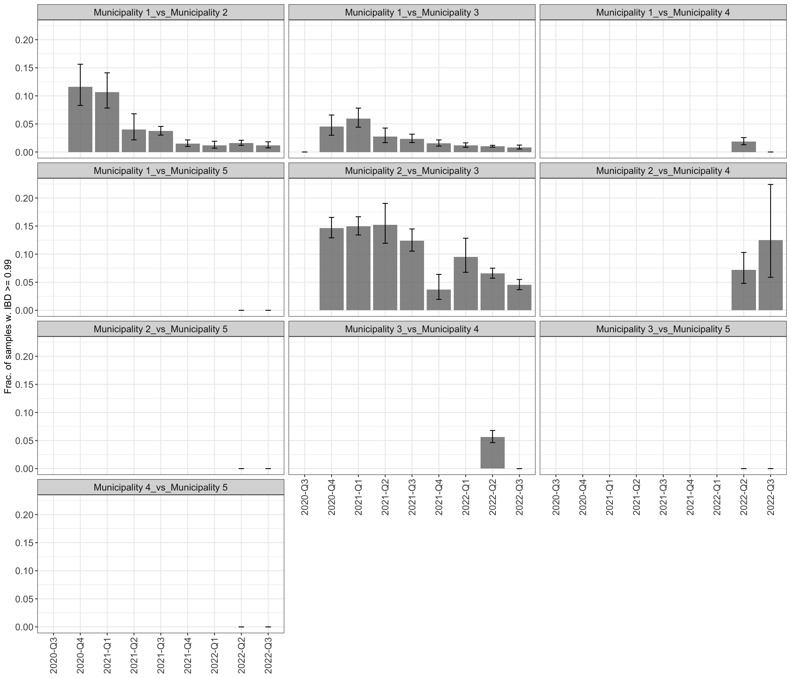
Figure 4: Bar plot of the fraction of highly related pairwise comparisons (IBD >= ibd_thres) between categories of Variable1 (panels) and Variable2 (x-axis). 95% confidence intervals are computed using a Fisher exact test.
Finally, let’s create PCoA and network plots summarizing the genetic relatedness between samples.
evectors_IBD = IBD_evectors(ampseq_object = ampseq_object,
                                relatedness_table = pairwise_relatedness,
                                k = length(unique(ampseq_object@metadata$Sample_id)),
                                Pop = 'Subnational_level2', q = 2)

col_vector = brewer.pal(5, 'Accent')

IBD_PCA = evectors_IBD$eigenvector %>% ggplot(aes(x = PC1, y = PC2, color = Subnational_level2))+
      geom_point(alpha = .7, size = 2) +
      stat_ellipse(level = .6)+
      scale_color_manual(values = col_vector)+
      theme_bw()+
      labs(x = paste0('1st PCo (', round(evectors_IBD$contrib[1],1), '%)'),
           y = paste0('2nd PCo (', round(evectors_IBD$contrib[2],1), '%)'),
           color = 'Countries')
IBD_PCA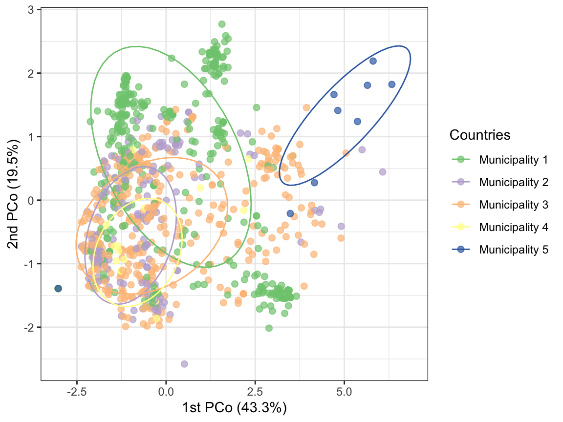
Figure 5: Principal coordinate analysis (PCoA) based on the inverse of genetic relatedness (1 - IBD). Colors are randomly assigned based on the categories of Variable1. Each dot represents a sample.
plot_network(pairwise_relatedness,
             threshold = 0.99,
             metadata = ampseq_object@metadata,
             sample_id = 'Sample_id',
             group_by = 'Subnational_level2',
             levels = levels(as.factor(
               ampseq_object@metadata[['Subnational_level2']])),
             colors = col_vector
             )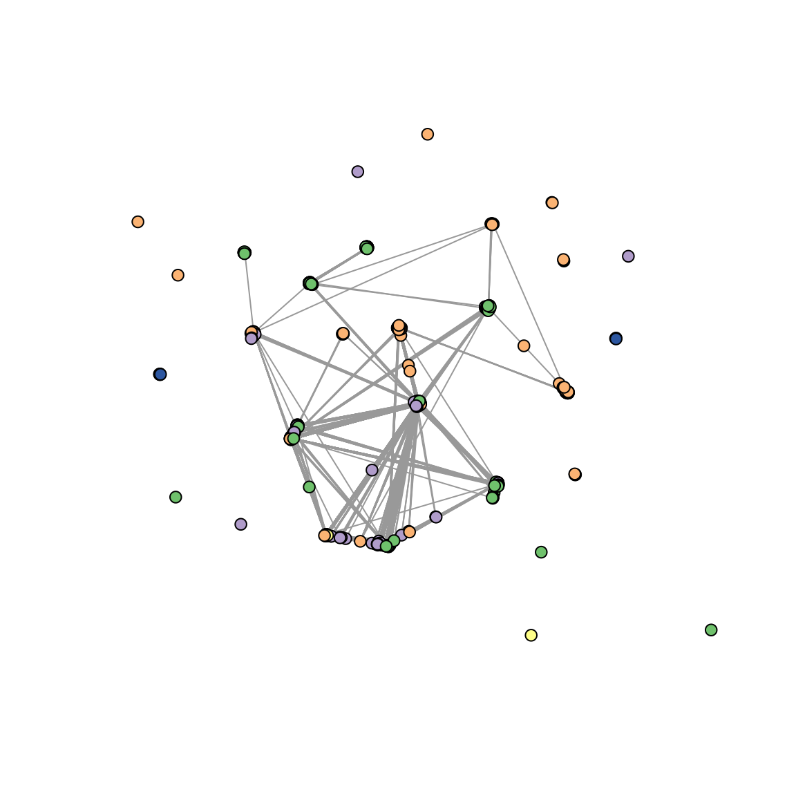
Figure 6: Network representation of pairwise genetic relatedness (IBD), Colors are randomly assigned based on the categories of Variable1. Each dot represents a sample and the lines connect samples with IBD >= ibd_thres.
## $network_object
## IGRAPH eb1377a UN-- 1146 44031 --
## + attr: name (v/c)
## + edges from eb1377a (vertex names):
##  [1] ID00001--ID00002 ID00001--ID00003 ID00001--ID00007 ID00001--ID00008
##  [5] ID00001--ID00009 ID00001--ID00010 ID00001--ID00011 ID00001--ID00014
##  [9] ID00001--ID00015 ID00001--ID00019 ID00001--ID00020 ID00001--ID00023
## [13] ID00001--ID00024 ID00001--ID00027 ID00001--ID00028 ID00001--ID00029
## [17] ID00001--ID00032 ID00001--ID00040 ID00001--ID00042 ID00001--ID00044
## [21] ID00001--ID00046 ID00001--ID00048 ID00001--ID00050 ID00001--ID00252
## [25] ID00001--ID00255 ID00001--ID00257 ID00001--ID00260 ID00001--ID00816
## [29] ID00001--ID00817 ID00001--ID00818 ID00001--ID00819 ID00001--ID00820
## + ... omitted several edges
##
## $plot_network
## NULL