Complexity of infection (COI)
Paulo Manrique
In malaria epidemiology, the term polyclonality represents the co-occurrence of two or more different parasite clones (e.g., haplotypes) within an infected individual. Polyclonality may occur due to the concurrent transmission of multiple parasite haplotypes from the same mosquito bite (co-infection) or the acquisition of different haplotypes through independent bites (super-infection). Both processes are related to the intensity of transmission. In low transmission settings, there are few infective bites and therefore little chance for super-infections or co-infections to occur. Most infections are therefore monoclonal. On the other hand, when conditions favor an increase in mosquito prevalence and human-mosquito interaction, super-infections and co-infections become more likely, generating an increase in the prevalence of polyclonal infections. Polyclonality rate is therefore generally considered a positive correlate of malaria transmission intensity (although other features such as case importation or relapse behavior in P. vivax may modify this relationship).
Differentiating monoclonal and polyclonal infections
There are different ways to differentiate between monoclonal and polyclonal infections and/or define the number of strains present in a sample. An easy and widely used way to differentiate between monoclonal and polyclonal infections is based on the number of heterozygous loci within the sample (\(N_{HetLoci}\)),. By using a pre-defined threshold (e.g., \(N_{HetLoci} \ge 1\)), samples are classified as polyclonal if they meet or exceed the threshold and classified as monoclonal if not. That definition is correct when working with a small number of loci, and de-novo mutations and genotyping errors are not frequent for those loci. When working with whole-genome or amplicon sequencing (microhaplotype) information, a sample can contain some heterozygous loci as a product of the diversification of the parasite population within the infection (de-novo mutations that occurs in the human or in the mosquito) or due to genotyping errors that occurs during amplification steps (sWGA, PCR1, or PCR2). For this reason, other metrics have been proposed to infer polyclonality. One simple metric is the fraction of heterozygous loci per sample (\(p_{Het_{(i)}}\)), defined as:
\[\text{Frac_HetLoci }(p_{Het_{(i)}}) =
N_{HetLoci_{(i)}} /N_{(i)}\]\(N_{HetLoci_{(i)}}\) represents the number
of heterozygous sites for sample \(i\)
and \(N_{(i)}\) represents the total
number of observed sites for sample \(i\).
Another metric used to infer polyclonality is the within-host divergence
(\(F_{WS_{(i)}}\)) index, defined as
follows:
\[F_{WS_{(i)}} = \displaystyle{\sum_{j = 1}^{n}{(1 - \frac{H_{W_j}}{H_{exp_{(j)}}})}}\]
\(H_{W_j}\) represents the within-host heterozygosity:
\[H_{W_j} = 1 - \displaystyle{\sum_{a = 1}^{b_j}{(\frac{({rd}_{a}^{j})}{RD_j})^2}}\]
Here, for each sample (\(i\)), \(rd_a^j\) represents the allele \(a\) observed at locus \(j\), \(b_j\) represents the total number of alleles observed at locus \(j\), and \(RD_j\) represents the total read-depth observed at locus \(j\).
\(H_{exp_{(j)}}\) is the within-population heterozygosity for locus \(j\):
\[H_{exp_{(j)}} = 1 - \displaystyle{\sum{p_j^2}}\]
Here, \(p_j\) represents the frequency of each of the alleles observed at locus \(j\) at the population level.
Another way to distinguish between monoclonal and polyclonal samples is to directly estimate the number of strains in each sample (i.e., define the ‘complexity of the infection’ (COI)). Samples with COI equal to 1 are monoclonal, and samples with greater values of COI are polyclonal. The easiest way to define the COI is to assume that it is equal to the maximum number of alleles (\(\text{max_nAlleles}\)) observed at any of the loci in the sample. More sophisticated approaches based on Markov Chain Monte Carlo (MCMC) methods also exist to estimate COI from biallelic and multiallelic loci, but these methods are not currently incorporated in the workflow.
In the current workflow, the user is able to set their own criteria
to distinguish between monoclonal and polyclonal samples based on the
combination of the metrics mentioned above. These criteria are set via
the parameter poly_formula (default
"poly_formula": "NHetLoci>1").
- First load libraries and functions in R:
source('~/Documents/Github/intro_to_genomic_surveillance/docs/functions_and_libraries/amplseq_required_libraries.R')
source('~/Documents/Github/intro_to_genomic_surveillance/docs/functions_and_libraries/amplseq_functions.R')
#sourceCpp('~/Documents/Github/intro_to_genomic_surveillance/docs/functions_and_libraries/hmmloglikelihood.cpp')- Read the ampseq_object in excel format:
ampseq_object = read_ampseq(file = '~/Documents/Github/intro_to_genomic_surveillance/docs/data/Pviv_example/Pviv_ampseq_filtered2.xlsx',
format = 'excel')- Identify polyclonal infections by Country
poly_by_Country = get_polygenomic(ampseq_object = ampseq_object,
                                   strata = 'Country',
                                   update_popsummary = FALSE,
                                   na.rm = T,
                                   filters = NULL,
                                   poly_quantile = 0.75,
                                   poly_formula = "NHetLoci > 1")
## [1] "Filter NHetLoci > 1 will be applied"In the following plot you can inspect the distribution of the fraction of heterozygous loci by sample (Frac_HetLoci), within-host divergence (Fws), and the maximum number of alleles found in a sample at any locus.
poly_by_Country$plot_fracHet_vs_Fws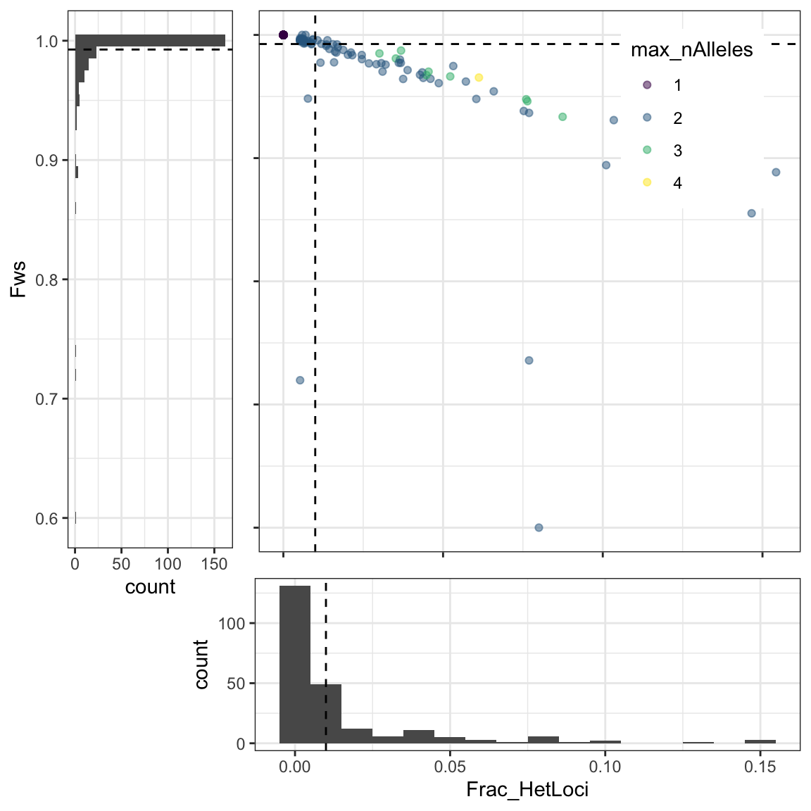
Figure 1: Distribution of the fraction of heterozygous loci by sample (fracHetLoci), within-host divergence (Fws), and the maximum number of alleles found in a sample at any locus. Dotted lines represent the quantiles defined by the poly_quantile argument in Terra.
All metrics are shown at the sample level in the following table. Information specifying which loci show heterozygosity in each sample is also presented.
poly_by_Country$coi_bySample %>% DT::datatable(extensions = 'Buttons',
                options = list(dom = 'Blfrtip',
                  buttons = c('csv', 'excel')))
The proportion of samples which show heterozygosity at each locus is specified below:
poly_by_Country$coi_byLoci %>% DT::datatable(extensions = 'Buttons',
                options = list(dom = 'Blfrtip',
                  buttons = c('csv', 'excel')))
Proportion of polyclonal infections by Country
The proportion of polyclonal infections by each category of the Variable1 is presented in the following table and figure.
poly_by_Country$pop_summary %>% DT::datatable(extensions = 'Buttons',
                options = list(dom = 'Blfrtip',
                  buttons = c('csv', 'excel')))
Plot the fraction of polyclonal samples per Country
plot_poly_by_pop = poly_by_Country$pop_summary %>%
      ggplot(aes(x = factor(pop,
                            levels = c(unique(poly_by_Country$pop_summary$pop)[unique(poly_by_Country$pop_summary$pop) != 'Total'], "Total")),
                 y = prop_poly,
                 fill = factor(pop,
                               levels = c(unique(poly_by_Country$pop_summary$pop)[unique(poly_by_Country$pop_summary$pop) != 'Total'], "Total"))))+
      geom_col(alpha = .6) +
      geom_errorbar(aes(ymin = prop_poly_lower, ymax = prop_poly_upper), width = .2)+
      theme_bw() +
      labs(title = "Frequency of polyclonal infections",
           y = "Frecquency") +
      scale_fill_manual(values = c('firebrick', 'dodgerblue', 'green4', 'gold3', "gray30"))+
      theme(axis.text = element_text(size = 12),
            axis.title = element_blank(),
            legend.position = "none",
            axis.text.x = element_text(angle = 90, vjust = 0.5))
fig2.height = 2.5 + max(round(nchar(as.character(unique(plot_poly_by_pop$data$pop)))/10, 0))
fig2.width = 1*length(unique(plot_poly_by_pop$data$pop))plot_poly_by_pop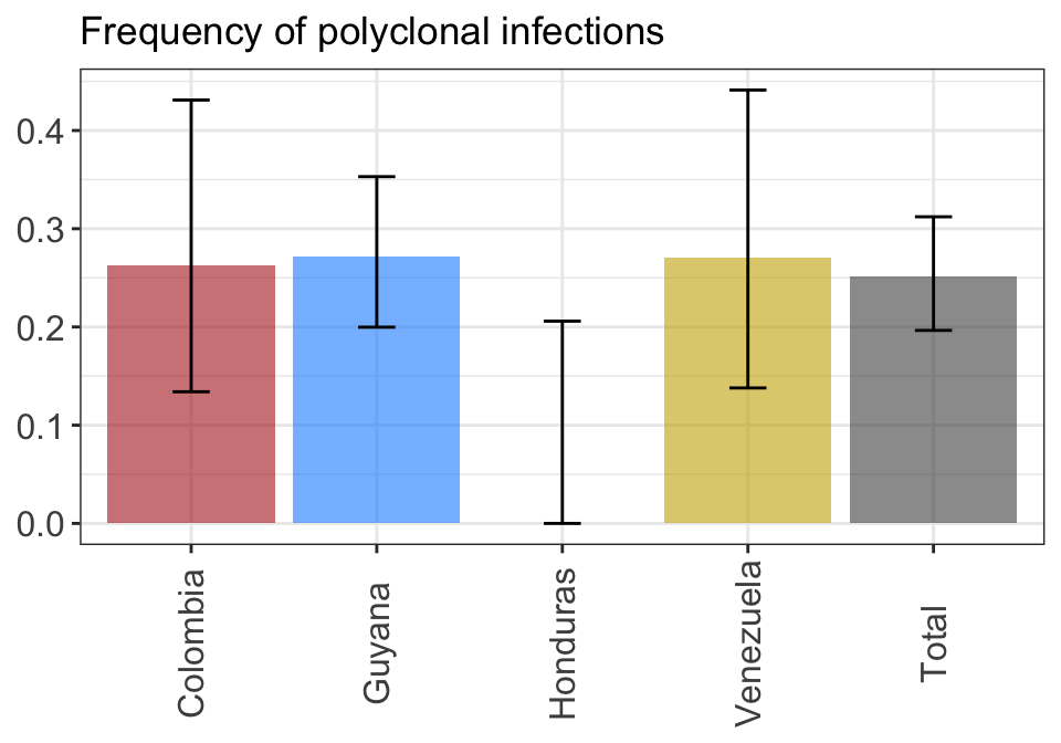
Figure 2: Proportions of polyclonal infections by Variable1. 95% confidence intervals are computed using a Fisher exact test.
Add information to the ampseq object and save
ampseq_object@metadata = left_join(ampseq_object@metadata,
                                   poly_by_Country$coi_bySample,
                                   by = 'Sample_id'
                                   )

ampseq_object@loci_performance = left_join(ampseq_object@loci_performance,
                                           poly_by_Country$coi_byLoci,
                                           by = join_by(loci == locus)
                                           )

# As an Excel file

write_ampseq(ampseq_object, format = 'excel', name = '~/Documents/Github/intro_to_genomic_surveillance/docs/data/Pviv_example/Pviv_ampseq_filtered3.xlsx')

# As csv files

write_ampseq(ampseq_object, format = 'csv', name = '~/Documents/Github/intro_to_genomic_surveillance/docs/data/Pviv_example/Pviv_ampseq_filtered3')
Polyclonal infections in P. falciparum
- Read the ampseq_object in excel format:
pfal_ampseq_object = read_ampseq(file = '~/Documents/Github/intro_to_genomic_surveillance/docs/data/Pfal_example/Pfal_ampseq_filtered',
format = 'csv')- Identify polyclonal infections by Subnational_level2
poly_by_snl2 = get_polygenomic(ampseq_object = pfal_ampseq_object,
                                   strata = 'Subnational_level2',
                                   update_popsummary = FALSE,
                                   na.rm = T,
                                   filters = NULL,
                                   poly_quantile = 0.75,
                                   poly_formula = "NHetLoci > 1")
## [1] "Filter NHetLoci > 1 will be applied"In the following plot you can inspect the distribution of the fraction of heterozygous loci by sample (Frac_HetLoci), within-host divergence (Fws), and the maximum number of alleles found in a sample at any locus.
poly_by_snl2$plot_fracHet_vs_Fws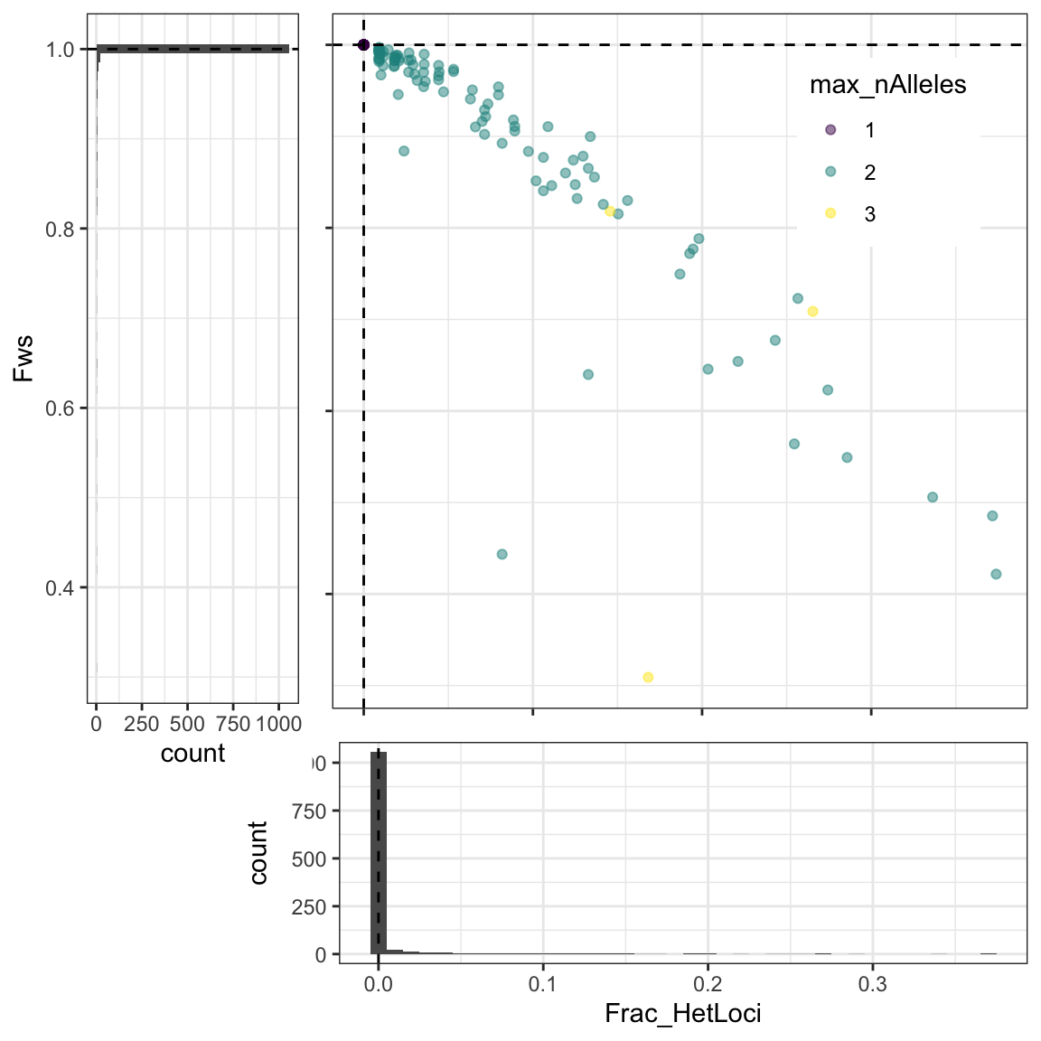
Figure 1: Distribution of the fraction of heterozygous loci by sample (fracHetLoci), within-host divergence (Fws), and the maximum number of alleles found in a sample at any locus. Dotted lines represent the quantiles defined by the poly_quantile argument in Terra.
All metrics are shown at the sample level in the following table. Information specifying which loci show heterozygosity in each sample is also presented.
poly_by_snl2$coi_bySample %>% DT::datatable(extensions = 'Buttons',
                options = list(dom = 'Blfrtip',
                  buttons = c('csv', 'excel')))
The proportion of samples which show heterozygosity at each locus is specified below:
poly_by_snl2$coi_byLoci %>% DT::datatable(extensions = 'Buttons',
                options = list(dom = 'Blfrtip',
                  buttons = c('csv', 'excel')))
Proportion of polyclonal infections by Subnational_level2
The proportion of polyclonal infections by each category of the Variable1 is presented in the following table and figure.
poly_by_snl2$pop_summary %>% DT::datatable(extensions = 'Buttons',
                options = list(dom = 'Blfrtip',
                  buttons = c('csv', 'excel')))
Plot the fraction of polyclonal samples per Country
plot_poly_by_snl2 = poly_by_snl2$pop_summary %>%
      ggplot(aes(x = factor(pop,
                            levels = c(unique(poly_by_snl2$pop_summary$pop)[unique(poly_by_snl2$pop_summary$pop) != 'Total'], "Total")),
                 y = prop_poly,
                 fill = factor(pop,
                               levels = c(unique(poly_by_snl2$pop_summary$pop)[unique(poly_by_snl2$pop_summary$pop) != 'Total'], "Total"))))+
      geom_col(alpha = .6) +
      geom_errorbar(aes(ymin = prop_poly_lower, ymax = prop_poly_upper), width = .2)+
      theme_bw() +
      labs(title = "Frequency of polyclonal infections",
           y = "Frecquency") +
      scale_fill_manual(values = c('firebrick', 'dodgerblue', 'green4', 'gold3', 'orange', "gray30"))+
      theme(axis.text = element_text(size = 12),
            axis.title = element_blank(),
            legend.position = "none",
            axis.text.x = element_text(angle = 90, vjust = 0.5))
fig2.height = 2.5 + max(round(nchar(as.character(unique(plot_poly_by_snl2$data$pop)))/10, 0))
fig2.width = 1*length(unique(plot_poly_by_snl2$data$pop))plot_poly_by_snl2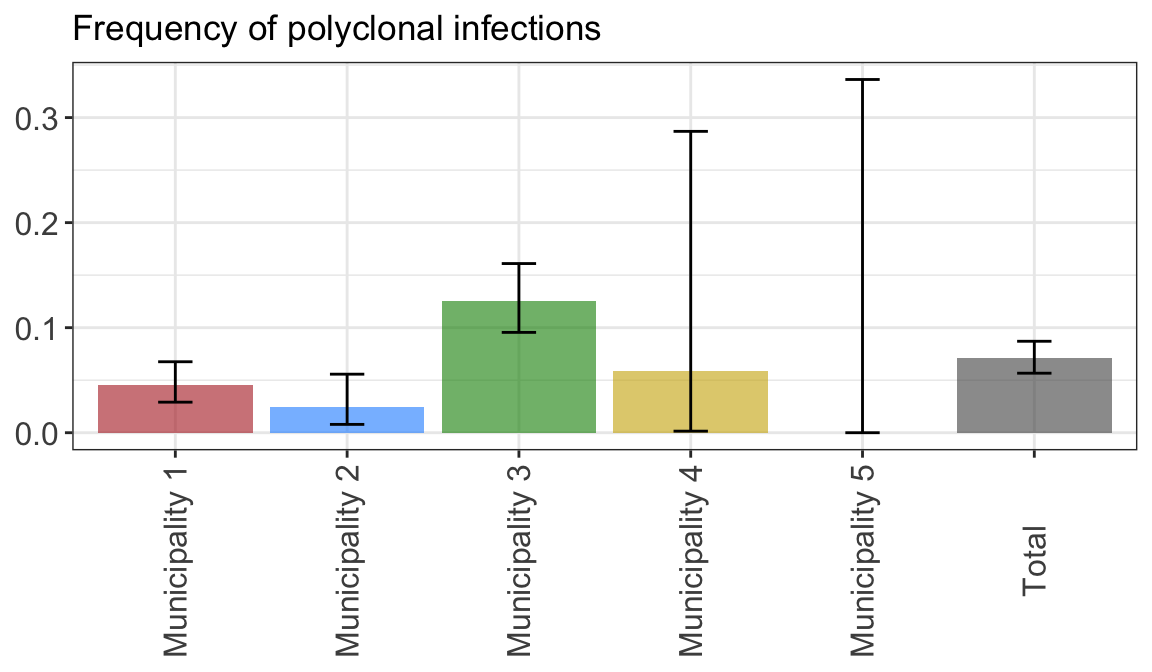
Figure 2: Proportions of polyclonal infections by Variable1. 95% confidence intervals are computed using a Fisher exact test.
Proportion of polyclonal infections by Subnational_level2 and Quarter_of_Collection
The proportion of polyclonal infections by each category of Variable1 and Variable2 is presented in the following table and figure.
pfal_ampseq_object@metadata[['snl2_qc']] =
  paste(pfal_ampseq_object@metadata[['Subnational_level2']],
        pfal_ampseq_object@metadata[['Quarter_of_Collection']], sep = '::')

poly_by_snl2_qc = get_polygenomic(ampseq_object = pfal_ampseq_object,
                                  strata = "snl2_qc",
                                  update_popsummary = F,
                                  na.rm = TRUE,
                                  filters = NULL,
                                  poly_quantile = .75,
                                  poly_formula = "NHetLoci > 1"
                                  )
## [1] "Filter NHetLoci > 1 will be applied"poly_by_snl2_qc$pop_summary %>% DT::datatable(extensions = 'Buttons',
options = list(dom = 'Blfrtip',
buttons = c('csv', 'excel')))plot_poly_by_snl2_qc = poly_by_snl2_qc$pop_summary %>%
filter(pop != 'Total')%>%
mutate(
Subnational_level2 = stringr::str_split(pop, '::', simplify = TRUE)[,1],
Quarter_of_Collection = stringr::str_split(pop, '::', simplify = TRUE)[,2],
prop_poly_lower = case_when(
prop_poly == 0 ~ 0,
prop_poly != 0 ~ prop_poly_lower),
prop_poly_upper = case_when(
prop_poly == 0 ~ 0,
prop_poly != 0 ~ prop_poly_upper)
)%>%
ggplot(aes(x = Quarter_of_Collection,
y = prop_poly,
ymin = prop_poly_lower,
ymax = prop_poly_upper,
fill = Subnational_level2))+
geom_col()+
geom_errorbar(width = .2)+
facet_wrap(~Subnational_level2, ncol = 3)+
theme_bw()+
scale_fill_manual(values = c('firebrick', 'dodgerblue', 'green4', 'gold3', 'orange'))+
labs(title = 'Temporal change of the proportion of polyclonal infections',
y = "Polyclonal infections",
x = "Quarter of Collection")+
theme(axis.text.x = element_text(angle = 90, vjust = 0.5),
legend.position = "none")plot_poly_by_snl2_qc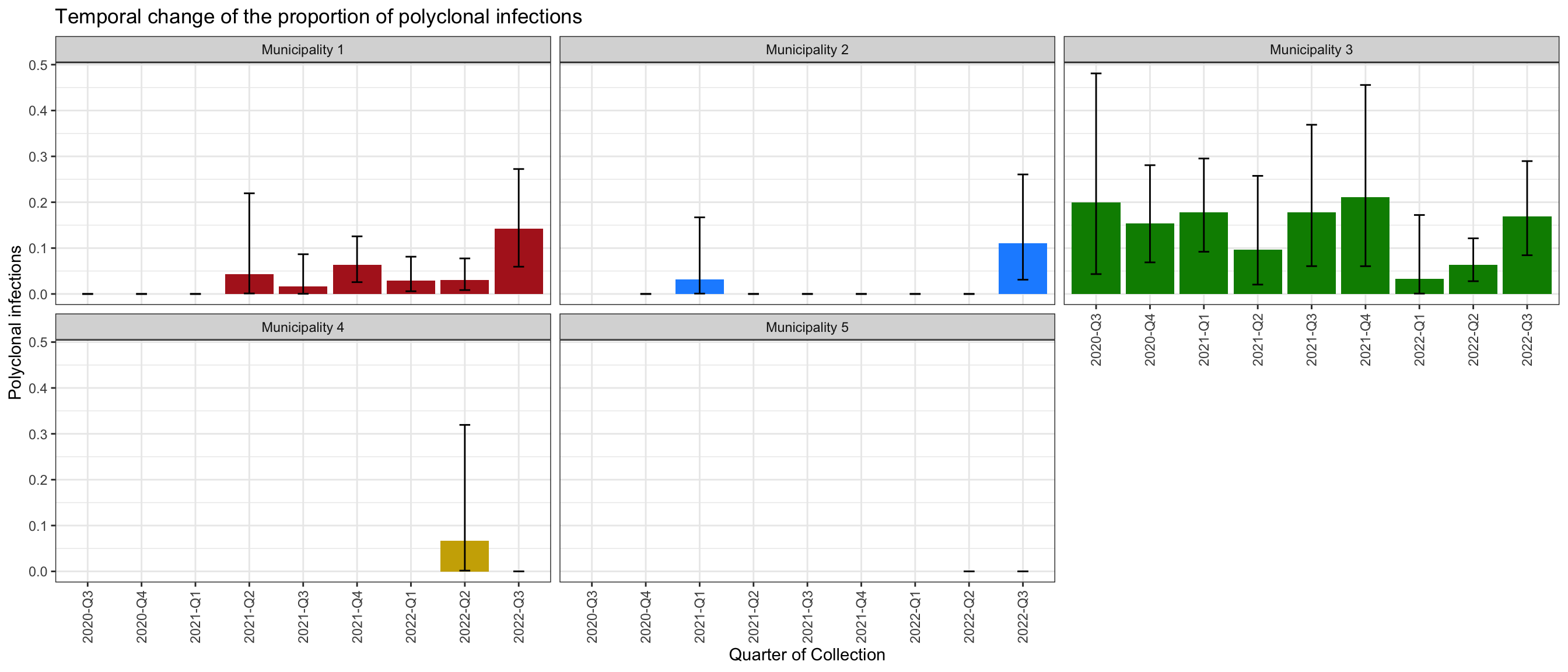
Figure 3: Proportions of polyclonal infections by Variable1. 95% confidence intervals are computed using a Fisher exact test.