Drug Resistance Surveillance
Paulo Manrique
Surveillance of polymorphisms or allelic variants associated with resistance against antimalarials is an important public health objective. Therefore most amplicon panels include several markers against genes that have polymorphisms associated with antimalarial resistance (i.e. AMPLseq includes 9 markers within 5 genes). This tutorial identifies the different haplotypes of these genes present in our data set, and we will determine the frequency of each haplotype in each category of two Variables of interest.
Upload libraries, functions and data
source('~/Documents/Github/intro_to_genomic_surveillance/docs/functions_and_libraries/amplseq_required_libraries.R')
source('~/Documents/Github/intro_to_genomic_surveillance/docs/functions_and_libraries/amplseq_functions.R')
#sourceCpp('~/Documents/Github/intro_to_genomic_surveillance/docs/functions_and_libraries/hmmloglikelihood.cpp')
Upload the data in ampseq format from the file
Pfal_ampseq_filtered.xlsx
ampseq_object = read_ampseq('~/Documents/Github/intro_to_genomic_surveillance/docs/data/Pfal_example/Pfal_ampseq_filtered.xlsx', format = 'excel')Inspect the metadata, and gnerate a bar plot of the number of sequenced samples by Subnational_level2, and Quarter_of_Collection
# Define the temporal unit of analysis
dates = sort(unique(ampseq_object@metadata$Quarter_of_Collection))

# Define the geographic unite of analysis
pop_levels = levels(as.factor(ampseq_object@metadata$Subnational_level2))
pop_colors = c("firebrick3", "dodgerblue3", "gold3", "darkseagreen3", "lightsalmon2")

plot_temporal_collection_of_samples = ampseq_object@metadata %>%
  filter(!is.na(Subnational_level2)) %>% # Remove samples with no geographic information (Controls)
  summarise(nsamples= n(), .by = c(Subnational_level2, Quarter_of_Collection))%>%
  ggplot(aes(x = Quarter_of_Collection, y = nsamples, fill = factor(Subnational_level2,
                                                              levels = pop_levels)))+
  geom_col()+
  theme_bw()+
  scale_fill_manual(values = pop_colors)+
  facet_wrap(.~factor(Subnational_level2,
                      levels = pop_levels),
             strip.position = "top", ncol = 5)+
  labs(title = 'Number of Samples collected over time',
       y = "Collected samples by PCD",
       x = "Quarter")+
  theme(axis.text.x = element_text(angle = 90, vjust = 0.5),
        legend.position =  "none")+
  scale_x_discrete(limits = dates)

plot_temporal_collection_of_samples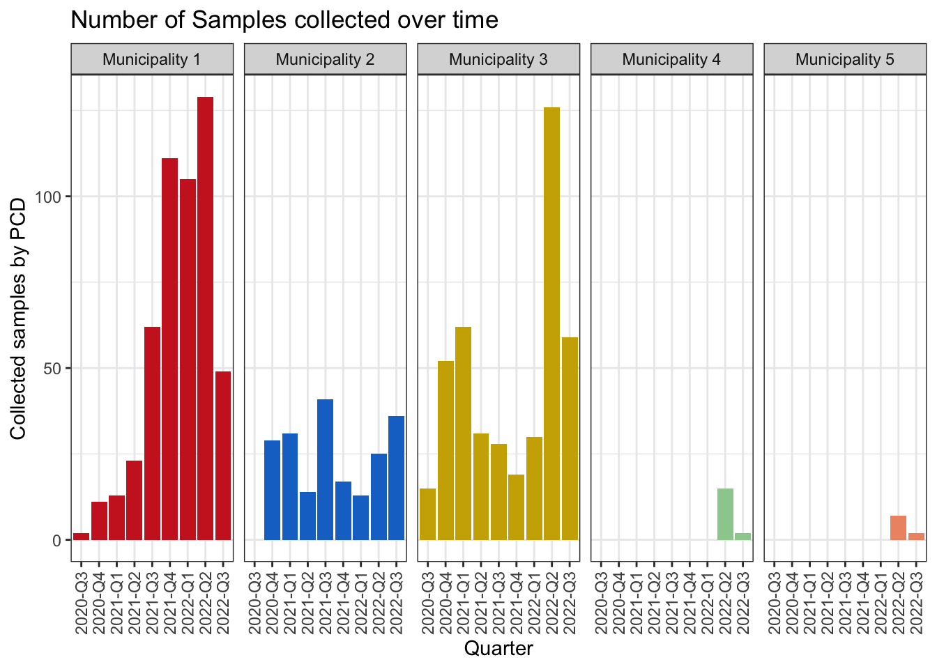
Drug resistance surveillance
The AMPLseq panel includes 5 genes (9 markers in total, some genes
are genotyped by more than one marker) that have polymorphisms
associated with antimalarial resistance. In this section we will
identify the different haplotypes of these genes present in our data
set, and we will determine the frequency of each haplotype in each study
area and in each quarter of the year. For this we will use the function
drug_resistant_haplotypes which has 7 arguments. The first
argument is the ampseq_object. The second is a table with
the reference alleles for each gene, and the polymorphisms associated
with resistance. The structure of this table is as follows:
\[\begin{array}{c|c:c:c} \text{Chromosome} & \text{Gene_ID} & \text{Description} & \text{Mutation} & \text{Anotation} \\ \text{Pf3D7_04_v3} & \text{PF3D7_0417200} & dhfr & \text{N51I} & \text{Pyrimethamine resistance} \\ ... \end{array}\]
Where the mutation describes the reference amino acid (sensitive to the drug), the position in the amino acid chain, and finally the amino acid associated with resistance.
The third and fourth arguments refer to the common name of the gene
(or the name by which it is identified in the markers table
in the ampseq_object) and the gene ID in the gff file of
the referential strain (in this case strain 3D7). The fifth and sixth
arguments are the .gff and .fasta files of the genome of the reference
strain, and the last argument, variables, is a vector that
has the columns of the metadata table that will be used to
define the subpopulations and generate the report graph. For this
particular example we will define as
variables = c('Sample_id', 'Subnational_level2', 'Quarter_of_Collection'),
where Sample_id, is the column that we will use to map the
data, Subnational_level2 is the column to define the area
of study, and Quarter_of_Collection defines the time
scale.
Let’s run the function drug_resistant_haplotypes:
gene_names = c('PfDHFR',
               'PfMDR1',
               'PfDHPS',
               'PfKelch13',
               'PF3D7_1447900')

gene_ids = c('PF3D7_0417200',
             'PF3D7_0523000',
             'PF3D7_0810800',
             'PF3D7_1343700',
             'PF3D7_1447900')

drugs = c('Artemisinin',
          'Chloroquine',
          'Pyrimethamine',
          'Sulfadoxine',
          'Lumefantrine',
          'Mefloquine')

drug_resistant_haplotypes_plot = drug_resistant_haplotypes(
  ampseq_object,
  reference_alleles = '~/Documents/Github/intro_to_genomic_surveillance/docs/reference/Pfal_3D7/drugR_alleles.csv',
  gene_names = gene_names,
  gene_ids = gene_ids,
  drugs = drugs,
  gff_file = "~/Documents/Github/intro_to_genomic_surveillance/docs/reference/Pfal_3D7/PlasmoDB-59_Pfalciparum3D7.gff",
  fasta_file = "~/Documents/Github/intro_to_genomic_surveillance/docs/reference/Pfal_3D7/PlasmoDB-59_Pfalciparum3D7_Genome.fasta",
  variables = c('Sample_id',
                'Subnational_level2',
                'Quarter_of_Collection'),
  Longitude = 'Longitude',
  Latitude = 'Latitude',
  na.var.rm = FALSE,
  na.hap.rm = TRUE,
  filters = c(
    'Subnational_level2;Municipality 1,Municipality 2,Municipality 3,Municipality 4,Municipality 5',
    'Quarter_of_Collection;2020-Q4,2021-Q1,2021-Q2,2021-Q3,2021-Q4,2022-Q1,2022-Q2,2022-Q3'),
  hap_color_palette = 'random')
## [1] "Uploading Resistant and Sensitive Alleles"
## [1] "Removing undesired categories based on var_filter"
## [1] "Defining haplotypes respect to a reference genome"
## [1] "Defining aa haplotypes and phenotipe respect to the presence of resistant alleles"
## [1] "Summarizing phenotype_table"
## [1] "Match Genotypes with Phenotypes"
## [1] "Handeling polyclonal samples for haplotype count"
## [1] "Adding metadata to haplotype counts"
## [1] "Summarizing haplotype counts"
## [1] "Calculating haplotype frequencies"
## [1] "haplotype_freq_barplot"
## [1] "haplotypes_freq_lineplot"
## [1] "Defining phenotypes based to drug of interest"
## [1] "drug_phenotype_barplot"
## [1] "drug_phenotyope_lineplot"
## [1] "Estimating frequency for drug resistant phenotypes"
## [1] "Transforming data to spatial points"
## [1] "i_drug_map"Outputs
Individual (sample-level) gene genotypes
Plasmodium parasites are haploid during the erythrocytic stage. However, multiple clone lineages can exist in the same infected individual. Some genes are amplified by multiple amplicons, making it hard to determine the haplotype of each individual clone (phasing or unique combination of alleles across several loci) in polyclonal infections. As such, in this report, we will use the term genotype to refer to the combination of alleles across loci in a sample, regardless of their clonal status. We will use the term haplotype to refer to the unique combination of alleles across loci in a gene for which we will calculate a population frequency.
In the cigar format the variant positions are based on the location of the mutation in the amplified region and not the position in the coding sequence, so this format does not directly indicate the consequences of the mutation in terms of amino acid change.
The workflow identifies the location of the mutations in the coding sequence, and based on that translates the base pair changes into amino acid changes. The annotation of the nucleotide and amino acid changes is based on the recommendations for the descriptions of variants from the Human Genome Variation Society with slight modifications. In the case of amino acid changes, we use the one letter code because it is shorter to show in tables and figures.
\[ \overbrace{c.\overbrace{152}^{\text{Position in coding sequence}}\underbrace{A}_{\text{Reference allele}}>\underbrace{T}_{\text{Observed allele}}}^{\text{Nucleotide change in coding region}} \equiv \underbrace{\overbrace{N}^{\text{Reference or Sensitive allele}}\underbrace{51}_{\text {Amino acid position}}\overbrace{I}^{\text{Observed Allele}}}_{\text{Amino acid change}} \]
The scheme above shows the notation for a nucleotide change in the coding sequence (left) and its equivalent amino acid change (right).
For a nucleotide change, the code starts with a c. which
makes reference to the coding sequence, then the number indicates the
position in the coding sequence of the gene, the first letter represents
the nucleotide in the reference strain, and finally the last letter
represents the observed nucleotide in the sample. If the DNA sequence of
the amplicon is 100% identical to the reference strain then the genotype
is written as follows c.(=).
Information on individual (sample-level) coding sequence polymorphism with respect to the reference strain is shown in the following table for each amplicon:
drug_resistant_haplotypes_plot$dna_mutations %>%
  DT::datatable(extensions = 'Buttons',
                options = list(
                  buttons = c('csv', 'excel')))
In the case of the amino acid change, allele codes are written such
that the letter to the left of the amino acid position represent the
reference strain allele. If the amino acid sequence of the amplicon is
100% identical to the reference strain then the genotype is written as
follows p.(=).
Information on individual (sample-level) amino acid polymorphism with respect to the reference strain is shown in the next table for each amplicon:
drug_resistant_haplotypes_plot$aa_mutations %>%
  DT::datatable(extensions = 'Buttons',
                options = list(dom = 'Blfrtip',
                  buttons = c('csv', 'excel')))
More often than not, the reference strain allele represents a
drug-sensitive phenotype. However, in some cases the reference strain
allele is itself a resistance-associated allele. In these cases, we
indicate the sensitive allele instead of the reference allele at the
left of the amino acid position in the code. The sensitive and
resistance-associated mutations are taken from the following article and
the information is incorporated into the workflow through the
reference_allele table in Terra. We use capital letters to
denote known resistance-associated mutations, and lowercase letters for
mutations not previously reported with respect to the reference strain.
Furthermore, if a sample contains two or more mutations, the haplotype
is determined by arranging the different mutations in ascending order in
relation to the positive DNA strand and the amino acid chain.
\[ \overbrace{\text{c.[47C>T;152A>T]}}^{\text{Nucleotide changes in coding region}} \equiv \underbrace{\overbrace{a16v}^{\text{Nonsynonymous polymorphism}\atop\text{with respect to reference strain}}\underbrace{N51I}_{\text{Known resistance-associated}\atop\text{mutation}}}_{\text{Amino acid changes}} \]
In the example above, there are two nonsynonymous mutations at positions 47 and 152 of the DNA coding sequence. The mutation at the first amino acid position has not been reported as resistance-associated, while the second one is a known resistance-associated mutation. If a resistance-associated mutation has been reported at a specific amino acid position, but we observe a change in the sample that has not been associated with resistance or not reported before, the first letter will be in uppercase and the second one in lowercase (e.g., \(N51a\)).
When an amplicon in a sample is heterozygous, then a slash (/) and a vertical bar (|) are used to separate the alleles in the DNA coding sequence and in the amino acid chain, respectively. If one gene is genotyped by two or more amplicons and one of them is heterozygous, the slash and vertical bar are only applicable to polymorphisms observed in the heterozygous amplicon. Moreover, all observed variants in the heterozygous amplicon are sorted in order of descending read depth (i.e. the better supported allele is indicated first).
\[ \overbrace{\overbrace{\text{c.[47C>T; 152A>T]/c.(=)}}^{1^{st}\text{ amplicon}} \text{; }\underbrace{\text{c.323G>A}}_{2^{nd}\text{ amplicon}}}^{\text{Nucleotide changes in coding region}} \equiv \underbrace{\overbrace{\text{a16v|a N51I|N}}^{1^{st}\text{ amplicon}} \underbrace{\text{ S108N}}_{2^{nd}\text{ amplicon}}}_{\text{Amino acid changes}} \]
In addition, as this genotype annotation could be confusing for people outside of the area of molecular biology and genetics, and as the presence of the resistant mutations does not directly indicate which drug the genotype might be resistant to, a table that matches the genotype and its likely phenotype is generated. In addition to showing which drug the mutations confer resistance, the phenotype output of the workflow also reports the number of resistance-associated mutations observed. Additional, resistance-unrelated mutations are also indicated by the phenotype output. Finally, the phenotype output also reports whether any amplicons or genes involve missing information (unsuccessful amplification).
The following scheme shows the annotated phenotype for the genotype of the gene \(pfdhfr\) (PF3D7_0417200):
\[ \overbrace{\text{a16v N51I C59C S108N I164I}}^{\text{Genotype}} \equiv \overbrace{\text{a16v polymorphism in gene PF3D7_0417200 respect to Reference Strain;} \atop \text{2 Pyrimethamine resistance-associated mutations}}^{\text{Likely Phenotype}} \]
As observed, the genotype contains 3 amino acid changes at positions 16, 51 and 108, the last two of which are associated to resistance to Pyrimethamine in previous studies. In the next scheme is an example of a genotype with missing data:
\[ \overbrace{\underbrace{\text{a16? N51? C59?}}_{\text{Amplicon PfDHFR_1}}\underbrace{\text{S108N I164I}}_{\text{Amplicon PfDHFR_2}}}^{\text{Genotype}} \equiv \overbrace{\text{Amplicon(s) PfDHFR_1 for gene PF3D7_0417200 did not amplify;} \atop \text{1 Pyrimethamine resistance mutation}}^{\text{Likely Phenotype}} \]
Question marks (?) represent missing information in the
genotype, placed after the amino acid positions found to be polymorphic
in other samples of the tested population or in previous studies (as
indicated in the reference_allele table). If none of the
amplicons amplify for a specific gene, the phenotype annotation will
read as Gene PF3D7_0417200 did not amplify. To enhance
readability across different samples and genotypes, the genotype of each
sample is written taking into account all polymorphic positions in the
data set or in previous studies (as indicated in the
reference_allele table).
Information on individual (sample-level) amino acid polymorphism with respect to the reference strain is shown in the next table for each gene of interest:
drug_resistant_haplotypes_plot$genotype_phenotype_table %>%
  DT::datatable(extensions = 'Buttons',
                options = list(dom = 'Blfrtip',
                  buttons = c('csv', 'excel')))
Haplotype frequency
The haplotype is defined as the unique combination of alleles across loci (variant sites across different amplicons) in a gene. In monoclonal samples, the genotype is equivalent to the haplotype as only one allele is observe at each locus.
For polyclonal samples, the complexity of infection (i.e., the number of strains in the sample) is defined based on the maximum number of alleles observed at any of the loci in the gene, and alleles in heterozygous loci are sorted in descending order of read depth. The order of the alleles in heterozygous loci is used to phase the haplotype:
\[ \overbrace{\underbrace{\text{a16v N51I|N C59C}}_{\text{Amplicon PfDHFR_1}}\underbrace{\text{S108N|S I164I}}_{\text{Amplicon PfDHFR_2}}}^{\text{Genotype}} \equiv \overbrace{\text{a16v N51 I C59C S108N I164I} \atop \text{a16v N51N C59C S108S I164I}}^{\text{Haplotypes}} \]
When different amplicons within a gene each show multiple alleles, and the number of alleles is different between these amplicons, the major allele on the locus with fewest alleles is used to impute the unknown/ambiguous haplotype(s) (haplotype with least read support).
\[ \overbrace{\underbrace{\text{a16v N51I|N C59C}}_{\text{Amplicon PfDHFR_1}}\underbrace{\text{ S108N|S|T I164I}}_{\text{Amplicon PfDHFR_2}}}^{\text{Genotype}} \equiv \overbrace{\text{a16v N51 I C59C S108N I164I} \\ \text{a16v N51N C59C S108S I164I} \\ \text{a16v N51 I C59C S108T I164I}}^{\text{Haplotypes}} \]
Finally, haplotypes observed in monoclonal and polyclonal infections have equal weights for calculating haplotype frequencies, so the denominator is the total number of haplotypes counted instead of the total number of infections.
The following table contains haplotype counts and frequencies (with 95% CI) for each category of Variable1 and Variable2:
drug_resistant_haplotypes_plot$haplotype_freq_barplot$data %>%
  DT::datatable(extensions = 'Buttons',
                options = list(dom = 'Blfrtip',
                  buttons = c('csv', 'excel')))
The next two figures shows the haplotype frequencies using a bar plot and a line plot with 95%CI
drug_resistant_haplotypes_plot$haplotype_freq_barplot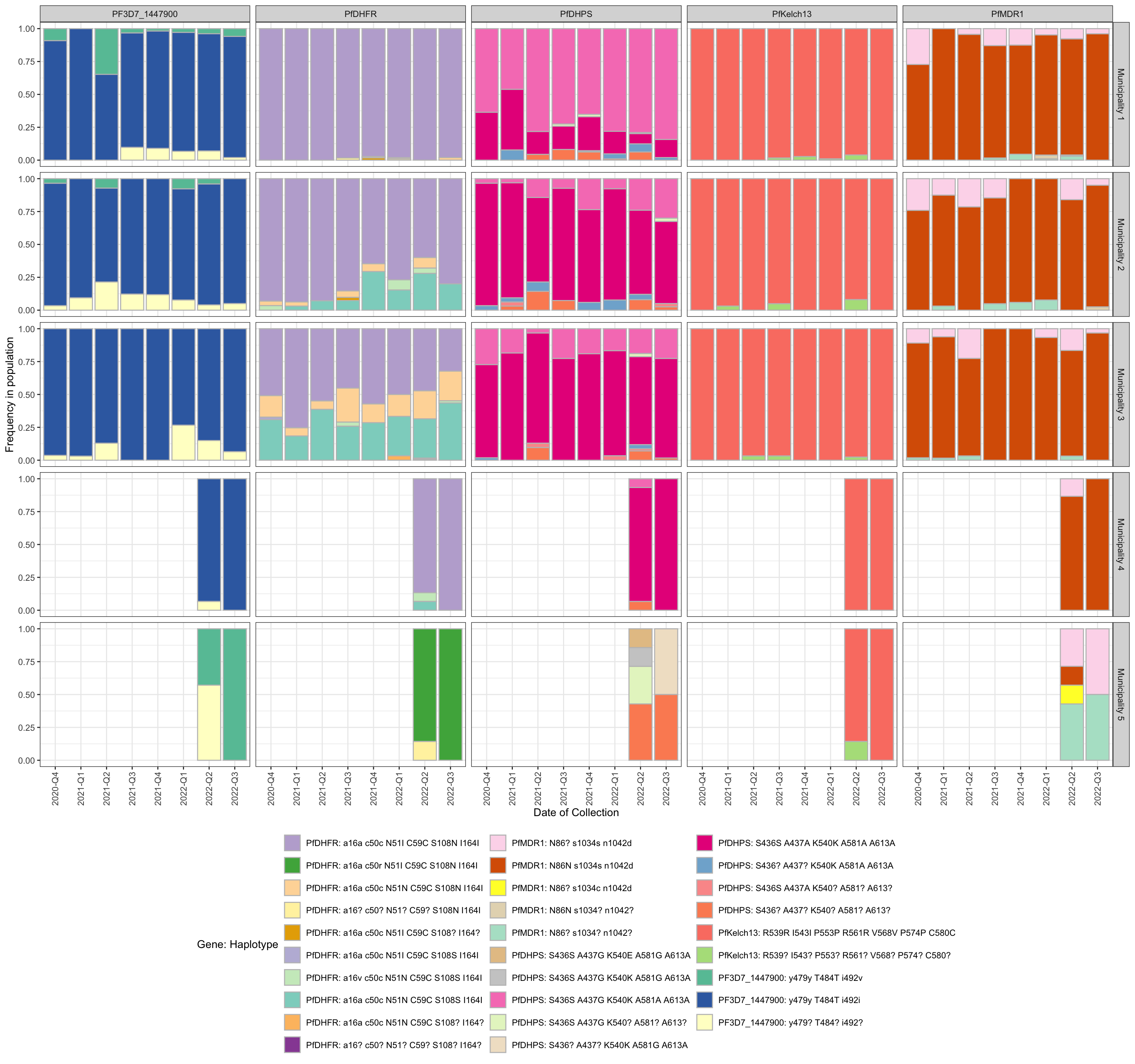
Figure 1: Bar plot showing the frequency of haplotypes of genes that carry mutations associated with resistance to Chloroquine, Lumefantrine, etc… (panels). y-axis shows the frequency in each population, x-axis shows the quarter of the year in which the sample was collected, horizontal sections correspond to the study areas, and vertical sections represents each Drug. If the user specifies ‘auto’ for the color scheme, blue indicates sensitive and red indicates the presence of one or more resistance-associated mutations. The intensity of red indicates the number of resistance-associated mutations. Finally, orange represents haplotypes carrying mutations with respect to the reference strain which have not been associated with resistance.
drug_resistant_haplotypes_plot$haplotypes_freq_lineplot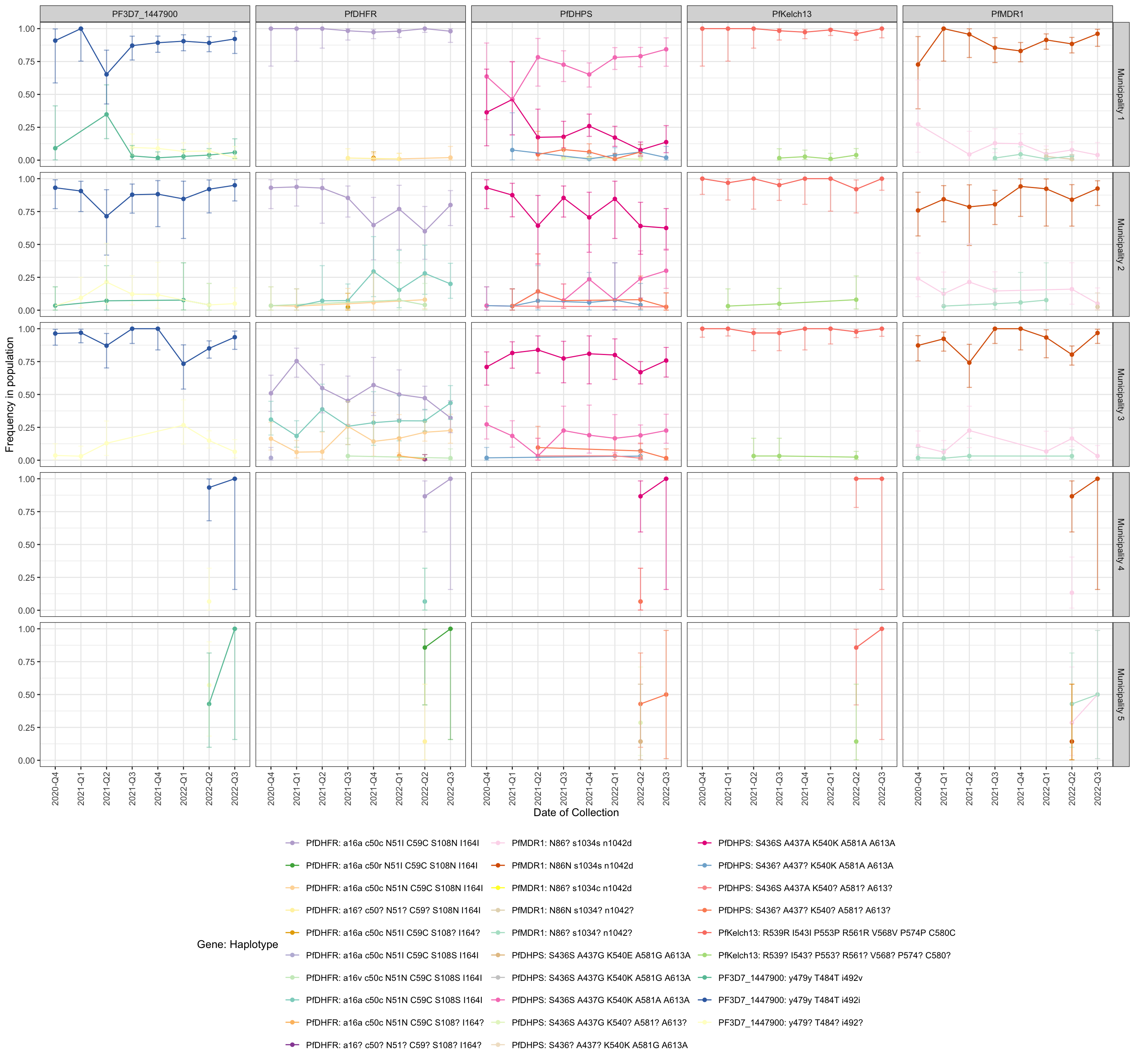
Figure 2: Line plot showing the frequency of haplotypes of genes that carry mutations associated with resistance to Chloroquine, Lumefantrine, etc… (panels). y-axis shows the frequency in each population, x-axis shows the quarter of the year in which the sample was collected, horizontal sections correspond to the study areas, and vertical sections represents each Gene. If the user specifies ‘auto’ for the color scheme, blue indicates sensitive and red indicates the presence of one or more resistance-associated mutations. The intensity of red indicates the number of resistance-associated mutations. Finally, orange represents haplotypes carrying mutations with respect to the reference strain which have not been associated with resistance.
Drug phenotypes
Resistance to a particular drug can be conferred by mutations in multiple different genes, which is why in this section, instead of using the gene as a unit of analysis we will use the drug of interest. In this way, for each drug in each sample we will define the possible phenotype based on the joint analysis of all the genes that have resistance-associated mutations to that particular drug.
For example, in the case of pyrimethamine, 7 mutations associated with resistance to this drug have been reported. Six of these mutations are found in the pfdhfr gene and one in the pfmdr2 gene. Therefore, to define the possible phenotype of this drug, the workflow will analyze the alleles present in each of these 7 positions in the sample. It will also report other mutations that occur in either of these two genes and whether amplification was unsuccessful for any of the amplicons.
Therefore, when no mutations are found, the phenotype is defined as follows:
\[ \begin{matrix}\overbrace{\text{a16v N51N C59C S108S I164I}}^{\text{Genotype for gene} \atop \text{pfdhfr: PF3D7_0417200}} \\ \underbrace{\text{y479y T484T i492i}}_{\text{Genotype for gene} \atop \text{pfmdr2: PF3D7_1447900}}\end{matrix} \implies \overbrace{\text{Sensitive phenotype based on gene(s) } \\ \text{PF3D7_0417200 and PF3D7_1447900}}^{\text{Phenotype}} \]
When at least one gene contains resistance-associated mutations or mutations with respect to the reference, the defined phenotype is:
\[ \begin{matrix}\overbrace{\text{a16v N51I C59C S108N I164I}}^{\text{Genotype for gene} \atop \text{pfdhfr: PF3D7_0417200}} \\ \underbrace{\text{y479y T484T i492v}}_{\text{Genotype for gene} \atop \text{pfmdr2: PF3D7_1447900}}\end{matrix} \implies \overbrace{\text{2 Pyrimethamine resistance mutations in gene PF3D7_0417200;} \\ \text{i492v polymorphism in gene PF3D7_1447900}}^{\text{Phenotype}} \]
In the case of partial or unsuccessful amplification of any of the genes:
\[ \begin{matrix}\overbrace{\text{a16v N51I C59C S108? I164?}}^{\text{Genotype for gene} \atop \text{pfdhfr: PF3D7_0417200}} \\ \underbrace{\text{y479? T484? i492?}}_{\text{Genotype for gene} \atop \text{pfmdr2: PF3D7_1447900}}\end{matrix} \implies \overbrace{\text{Partial haplotype: Amplicon(s) PfDHFR_2 for gene PF3D7_0417200 did not amplify} \\ \text{and Gene PF3D7_1447900 did not amplify}}^{\text{Phenotype}} \]
Information on individual (sample-level) phenotypes is shown in the next table for each drug of interest:
drug_resistant_haplotypes_plot$drug_phenotype_table %>%
  DT::datatable(extensions = 'Buttons',
                options = list(dom = 'Blfrtip',
                  buttons = c('csv', 'excel')))
For each drug the phenotypic profiles are classified into five categories:
- Sensitive Phenotype: All amplicons amplified and no mutations were
found with respect to the reference strain and the
reference_alleletable. - Polymorphism(s) with respect to the reference strain: At least one mutation with respect to the reference strain was found, but no resistance-associated mutations occur. Partial haplotypes are also included.
- Mutation(s) associated with a resistant phenotype: At least one resistance-associated mutations was found. Partial haplotypes are also included.
- Partial Haplotype: At least one amplicon has amplified and no mutations occur.
- Missing data: None of the amplicons amplified.
Finally, the prevalence of these categories in the population (defined by Variable1 and Variable2) is reported in the following table:
drug_resistant_haplotypes_plot$drug_phenotype_barplot$data %>%
  DT::datatable(extensions = 'Buttons',
                options = list(dom = 'Blfrtip',
                  buttons = c('csv', 'excel')))
The next three figures show the phenotype frequencies using a bar plot and a line plot with 95% CI, and a map of the geographic distribution of resistance phenotypes with respect to each drug of interest.
drug_resistant_haplotypes_plot$drug_phenotype_barplot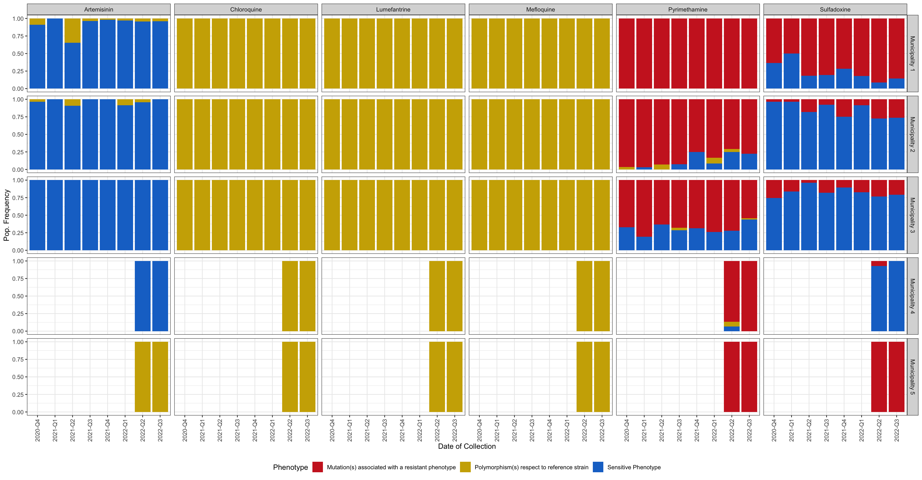
Figure 3: Bar plot showing the frequency of phenotypes (resistant vs. sensitive) classified based on amino acid changes in drug resistance-associated genes. y-axis shows the frequency in each population, x-axis shows the quarter of the year in which the sample was collected, horizontal sections correspond to the study areas, and vertical sections represents each Drug. Blue indicates sensitive and red indicates the presence of one or more resistance-associated mutations. Gold represents haplotypes carrying mutations with respect to the reference strain which have not been associated with resistance.
drug_resistant_haplotypes_plot$drug_phenotyope_lineplot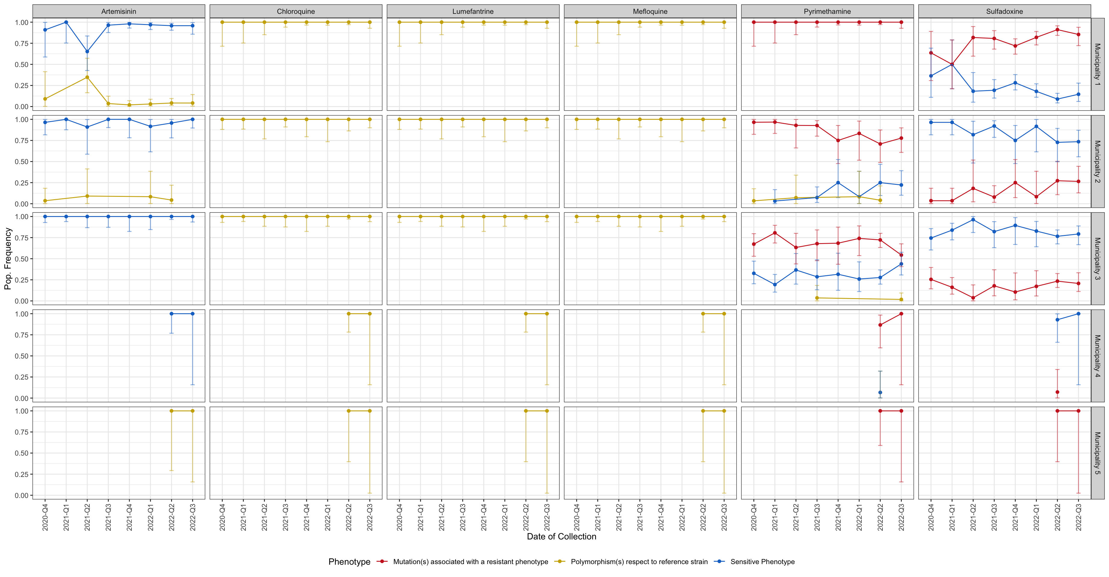
Figure 4: Line plot showing the frequency of phenotypes (resistant vs. sensitive) classified based on amino acid changes in drug resistance-associated genes. y-axis shows the frequency in each population, x-axis shows the quarter of the year in which the sample was collected, horizontal sections correspond to the study areas, and vertical sections represents each Drug. Blue indicates sensitive and red indicates the presence of one or more resistance-associated mutations. Gold represents haplotypes carrying mutations with respect to the reference strain which have not been associated with resistance
library(tmap)
tmap_mode('view')
drug_resistant_haplotypes_plot$i_drug_map