Content

Importing and handling tables in CIGAR format in R environment.
Preliminary sequencing yield by Run and Variable1.
Identification of potential genotyping errors.
Read depth yield per sample and locus.
Retention of loci and samples for subsequent analysis.

This tutorial is based on the output of the Dada2-based denoising pipeline. The main output (the cigar table) of the denoising pipeline has the following structure:

\(\begin{array}{c|c:c:c:c:c:c} \text{sampleID}&Gene_1,Allele_1&Gene_1,Allele_2&...&Gene_1,Allele_k&... & Gene_m, Allele_{k_m}\\ \hline ID_1 & \text{Read counts} &&& \\ \hdashline ... &&&&\\ \hdashline ID_n &&&& \end{array}\)

Where the \(Allele\) is coded in Pseudo-CIGAR format, typing “.” for the reference allele, \([0-9]*[A,T,C,G]\) for each point mutation observed, and \([0-9]*[D,I]=[A,T,C,G]*\) for indels (Insertions and Deletions). The numbers before the letters denotes the position in the amplicon where the polymorphism is located.

Documentation of the denoising pipeline can be found in the repository malaria-amplicon-pipeline, and the steps used to generate the inputs files for the current tutorial are in Intro to MHap-Analysis pipeline

Importing and handling tables in CIGAR format in R environment

Our first step will be to call all required packages and functions in the R environment:

source('/Users/pam3650/Documents/Github/MHap-Analysis/docs/functions_and_libraries/amplseq_required_libraries.R')
source('~/Documents/Github/MHap-Analysis/docs/functions_and_libraries/amplseq_functions.R')

In the previous section the Pseudo-CIGAR tables were stored in the computer using the following path structure:

"STUDYNAME/RUNNAME/dada2/run_dada2/CIGARVariants.out.tsv"

As this structure is maintained across different sequencing runs, we have created a function called read_cigar_tables that at least only requires two arguments: paths (name of the folder of the study or the STUDYNAME), and sample_id_pattern (a pattern string in the IDs of the samples that differentiate them from controls). In case you don’t want to differentiate samples from controls, set this argument equals to ".". For this particular example, the path will be "data/sequencing_data/" , while the pattern will be ".". In case all ".tvs" files are stored in one folder, you can use the argument cigar_files = list_of_files instead of the argument paths, where list_of_files is a vector with the names of all files we want to read.

## [1] "Cigar file ~/Documents/Github/MHap-Analysis/docs/data/Pviv_example/potential_markers.csv/dada2/run_dada2/CIGARVariants_Bfilter.out.tsv not found"
## [1] "asv2cigar file ~/Documents/Github/MHap-Analysis/docs/data/Pviv_example/potential_markers.csv/dada2/run_dada2/ASVTable.txt not found"
## [1] "asv_table file ~/Documents/Github/MHap-Analysis/docs/data/Pviv_example/potential_markers.csv/dada2/run_dada2/ASVTable.txt not found"
## [1] "asv_seqs file ~/Documents/Github/MHap-Analysis/docs/data/Pviv_example/potential_markers.csv/dada2/run_dada2/ASVSeqs.fasta not found"
## [1] "asv_seqs file ~/Documents/Github/MHap-Analysis/docs/data/Pviv_example/potential_markers.csv/dada2/run_dada2/zeroReadSamples.txt not found"
## [1] "Cigar file ~/Documents/Github/MHap-Analysis/docs/data/Pviv_example/Pviv_ampseq_filtered/dada2/run_dada2/CIGARVariants_Bfilter.out.tsv not found"
## [1] "asv2cigar file ~/Documents/Github/MHap-Analysis/docs/data/Pviv_example/Pviv_ampseq_filtered/dada2/run_dada2/ASVTable.txt not found"
## [1] "asv_table file ~/Documents/Github/MHap-Analysis/docs/data/Pviv_example/Pviv_ampseq_filtered/dada2/run_dada2/ASVTable.txt not found"
## [1] "asv_seqs file ~/Documents/Github/MHap-Analysis/docs/data/Pviv_example/Pviv_ampseq_filtered/dada2/run_dada2/ASVSeqs.fasta not found"
## [1] "asv_seqs file ~/Documents/Github/MHap-Analysis/docs/data/Pviv_example/Pviv_ampseq_filtered/dada2/run_dada2/zeroReadSamples.txt not found"
## [1] "Cigar file ~/Documents/Github/MHap-Analysis/docs/data/Pviv_example/Pviv_ampseq_filtered.xlsx/dada2/run_dada2/CIGARVariants_Bfilter.out.tsv not found"
## [1] "asv2cigar file ~/Documents/Github/MHap-Analysis/docs/data/Pviv_example/Pviv_ampseq_filtered.xlsx/dada2/run_dada2/ASVTable.txt not found"
## [1] "asv_table file ~/Documents/Github/MHap-Analysis/docs/data/Pviv_example/Pviv_ampseq_filtered.xlsx/dada2/run_dada2/ASVTable.txt not found"
## [1] "asv_seqs file ~/Documents/Github/MHap-Analysis/docs/data/Pviv_example/Pviv_ampseq_filtered.xlsx/dada2/run_dada2/ASVSeqs.fasta not found"
## [1] "asv_seqs file ~/Documents/Github/MHap-Analysis/docs/data/Pviv_example/Pviv_ampseq_filtered.xlsx/dada2/run_dada2/zeroReadSamples.txt not found"
## [1] "Cigar file ~/Documents/Github/MHap-Analysis/docs/data/Pviv_example/Pviv_ampseq_filtered2/dada2/run_dada2/CIGARVariants_Bfilter.out.tsv not found"
## [1] "asv2cigar file ~/Documents/Github/MHap-Analysis/docs/data/Pviv_example/Pviv_ampseq_filtered2/dada2/run_dada2/ASVTable.txt not found"
## [1] "asv_table file ~/Documents/Github/MHap-Analysis/docs/data/Pviv_example/Pviv_ampseq_filtered2/dada2/run_dada2/ASVTable.txt not found"
## [1] "asv_seqs file ~/Documents/Github/MHap-Analysis/docs/data/Pviv_example/Pviv_ampseq_filtered2/dada2/run_dada2/ASVSeqs.fasta not found"
## [1] "asv_seqs file ~/Documents/Github/MHap-Analysis/docs/data/Pviv_example/Pviv_ampseq_filtered2/dada2/run_dada2/zeroReadSamples.txt not found"
## [1] "Cigar file ~/Documents/Github/MHap-Analysis/docs/data/Pviv_example/Pviv_ampseq_filtered2.xlsx/dada2/run_dada2/CIGARVariants_Bfilter.out.tsv not found"
## [1] "asv2cigar file ~/Documents/Github/MHap-Analysis/docs/data/Pviv_example/Pviv_ampseq_filtered2.xlsx/dada2/run_dada2/ASVTable.txt not found"
## [1] "asv_table file ~/Documents/Github/MHap-Analysis/docs/data/Pviv_example/Pviv_ampseq_filtered2.xlsx/dada2/run_dada2/ASVTable.txt not found"
## [1] "asv_seqs file ~/Documents/Github/MHap-Analysis/docs/data/Pviv_example/Pviv_ampseq_filtered2.xlsx/dada2/run_dada2/ASVSeqs.fasta not found"
## [1] "asv_seqs file ~/Documents/Github/MHap-Analysis/docs/data/Pviv_example/Pviv_ampseq_filtered2.xlsx/dada2/run_dada2/zeroReadSamples.txt not found"
## [1] "Cigar file ~/Documents/Github/MHap-Analysis/docs/data/Pviv_example/Pviv_ampseq_filtered3/dada2/run_dada2/CIGARVariants_Bfilter.out.tsv not found"
## [1] "asv2cigar file ~/Documents/Github/MHap-Analysis/docs/data/Pviv_example/Pviv_ampseq_filtered3/dada2/run_dada2/ASVTable.txt not found"
## [1] "asv_table file ~/Documents/Github/MHap-Analysis/docs/data/Pviv_example/Pviv_ampseq_filtered3/dada2/run_dada2/ASVTable.txt not found"
## [1] "asv_seqs file ~/Documents/Github/MHap-Analysis/docs/data/Pviv_example/Pviv_ampseq_filtered3/dada2/run_dada2/ASVSeqs.fasta not found"
## [1] "asv_seqs file ~/Documents/Github/MHap-Analysis/docs/data/Pviv_example/Pviv_ampseq_filtered3/dada2/run_dada2/zeroReadSamples.txt not found"
## [1] "Cigar file ~/Documents/Github/MHap-Analysis/docs/data/Pviv_example/Pviv_ampseq_filtered3.xlsx/dada2/run_dada2/CIGARVariants_Bfilter.out.tsv not found"
## [1] "asv2cigar file ~/Documents/Github/MHap-Analysis/docs/data/Pviv_example/Pviv_ampseq_filtered3.xlsx/dada2/run_dada2/ASVTable.txt not found"
## [1] "asv_table file ~/Documents/Github/MHap-Analysis/docs/data/Pviv_example/Pviv_ampseq_filtered3.xlsx/dada2/run_dada2/ASVTable.txt not found"
## [1] "asv_seqs file ~/Documents/Github/MHap-Analysis/docs/data/Pviv_example/Pviv_ampseq_filtered3.xlsx/dada2/run_dada2/ASVSeqs.fasta not found"
## [1] "asv_seqs file ~/Documents/Github/MHap-Analysis/docs/data/Pviv_example/Pviv_ampseq_filtered3.xlsx/dada2/run_dada2/zeroReadSamples.txt not found"

Use the function slotNames to visualize the slots that the cigar_object has:

slotNames(cigar_object)

## [1] "cigar_table" "metadata"    "asv_table"   "asv_seqs"

This function generates a S4 cigar object containing three data.frames and one list:

cigar_table, where genotyping information is stored in cigar format;
metadata table with 4 variables (columns), a) Sample_id which contains samples Id’s; b) run which contains the run number (or the name of the folter where the fastq’s for that run wehere stored), information that is useful for comparing performance across batches of samples; c) order_in_plate, useful to identify rare amplifications patterns in the plate; and d) typeofSamp which differentiates between controls and samples of interest.
asv_table that contains summary metrics of each asv and the corresponding cigar string.
asv_seqs which is the nucleotide sequence of each asv.

To view these slots use View(cigar_table@cigar_table) in the console.

NOTE: If there are duplicated samples, only the replicated with the highest read depth across all loci will be kept.

Adding Metadata

Metadata would come from different sources, sometimes the sample ID incorporates metadata in their coding system, other times metadata can be stored in a different table, having one column specifying the sample ID.

Inspect the metadata slot and check if the IDs tell you something about the procidence of the samples

View(cigar_object@metadata)

Samples that starts with SP comes from Colombia, samples that starts with G are fom Guyana, samples that starts with PF or contains GZ are from Honduras, and samples that starts with HRP are from Venezuela.

We can use the function mutate and a regular expression pattern in grepl to adding the country from where the sample was collected to the metadata. Also update the column typeofSamp, to be able to distinguish between samples of interest and controls

cigar_object@metadata %<>% mutate(
  typeofSamp = case_when(
    grepl('(^SP|^G|^PF|-GZ|^HRP)', Sample_id) ~ typeofSamp,
    !grepl('(^SP|^G|^PF|-GZ|^HRP)', Sample_id) ~ 'Controls'
  ),
  Country = case_when(
    grepl('^SP', Sample_id) ~ 'Colombia',
    grepl('^G', Sample_id) ~ 'Guyana',
    grepl('(^PF|-GZ)', Sample_id) ~ 'Honduras',
    grepl('^HRP', Sample_id) ~ 'Venezuela',
    .default = 'Controls'
  )
)

Use View again to visualize those changes.

The cigar_table is in wide format, and the alleles corresponding to the sample target are not in consecutive order. Because of that e are going to convert our cigar_table to a more manageable (easy to read for the user) format called ampseq format, where amplicons or genes are going to be in columns, samples in rows, and the allele in cigar format is going to be in each cell of the matrix together with the read count of that allele in the sample.

\(\begin{array}{c|c:c:c:c} \text{sampleID}&Gene_1&Gene_2&...& Gene_m\\ \hline ID_1 & Allele_{i_{i \in Alleles_{Gene_1}}}\text{:Read count} &&& \\ \hdashline ... &&&&\\ \hdashline ID_n &&&& \end{array}\)

For that purpose we are going to use the function cigar2ampseq. This function requires 4 arguments. First a cigar_object (containing the cigar_table and the metadata). Then markers, which is a table with the set of markers and their names (in a column named amplicon). This argument is optional, and in case is NULL, the name of the amplicons will be extracted from the columns in the cigar_object, but information regarding chormosome location (information required to estimate relatedness under the hmmIBD algorithm) and length of the amplicon will be missing. The next arguments are min_abd and min_ratio, which are the minimum abundance (minimum read count) required to call an allele and the minimum ratio between the minor and major alleles in a polyclonal sample. By default these two arguments are 10 and 0.1 respectively. The last argument is remove_controls, by default is FALSE, but if change to TRUE the information of the controls will be stored in a separated slot. Thus, this function automatically differentiate between controls and samples of interest, and its output is a ampseq_object S4 list with 11 slots: gt where the genotypic information of the samples of interest is stored in a ampseq format; the asv_table with summary metrics and the cigar strings for each asv (allele); the asv_seqs list that store the nucleotide sequence of each asv, the metadata of the samples of interest; controls with all the information of the controls; markers containing the information of the markers such as the chromosome location; and other empty slots required for the next steps such as loci_performance and pop_summary.

For the next steps we are going to convert the cigar_object into an ampseq_object in two different ways:

Keeping controls and all asvs observed in the data set.
Removing controls and asvs with less than 5 reads of support.

But first lest upload the information of the markers into the R environment:

markers = read.csv('~/Documents/Github/MHap-Analysis/docs/reference/Pviv_P01/PvGTSeq271_markersTable.csv')

Inspect the table using View() in the console.

ampseq_object_abd1 = cigar2ampseq(cigar_object, markers = markers, min_abd = 1, min_ratio = 0.001, remove_controls = F)
ampseq_object = cigar2ampseq(cigar_object, markers = markers, min_abd = 5, min_ratio = 0.1, remove_controls = T)

The table of the markers contains a list of 271 amplicons, however the samples were sequenced using only 249. Filter the ampseq objects using the function filter_loci

ampseq_object_abd1 = filter_loci(ampseq_object_abd1,
                                 v = grepl('249', ampseq_object_abd1@markers$Set))

ampseq_object = filter_loci(ampseq_object,
                                 v = grepl('249', ampseq_object_abd1@markers$Set))

Preliminary sequencing yield by Run and Country

Sample success is defined as the percentage of samples which amplify a specific percentage of loci given the allele detection coverage threshold or number of paired reads that support the allele or ASV in a sample. Here we are going to show 6 different coverage thresholds: 1, 5, 10, 20, 50, and 100 paired reads.

Overall sequencing yield

Measure the read coverage by using the function get_ReadDepth_coverage:

ReadDepth_coverage = get_ReadDepth_coverage(ampseq_object_abd1, variable = NULL)

For each sample, calculates how many loci has a read depth equals or greater than 1, 5, 10, 20, 50, or 100:

sample_performance = ReadDepth_coverage$plot_read_depth_heatmap$data %>%
    mutate(Read_depth = case_when(
      is.na(Read_depth) ~ 0,
      !is.na(Read_depth) ~ Read_depth
    )) %>%
    summarise(amplified_amplicons1 = sum(Read_depth >= 1)/nrow(ampseq_object_abd1@markers),
              amplified_amplicons5 = sum(Read_depth >= 5)/nrow(ampseq_object_abd1@markers),
              amplified_amplicons10 = sum(Read_depth >= 10)/nrow(ampseq_object_abd1@markers),
              amplified_amplicons20 = sum(Read_depth >= 20)/nrow(ampseq_object_abd1@markers),
              amplified_amplicons50 = sum(Read_depth >= 50)/nrow(ampseq_object_abd1@markers),
              amplified_amplicons100 = sum(Read_depth >= 100)/nrow(ampseq_object_abd1@markers),
              .by = Sample_id) %>%
    pivot_longer(cols = starts_with('amplified_amplicons'), values_to = 'AmpRate', names_to = 'Threshold') %>%
    mutate(Threshold = as.integer(gsub('amplified_amplicons', '', Threshold)))

Generate a plot showing the percentage of loci (amplicon or marker) which contains alleles that pass the thresholds in the x-axis, and the percentage of samples which amplify a specific percentage of loci given the allele detection thresholds in the y-axis. Include a vertical line that indicates samples that has amplify at least 50% of the loci with the especific read depth coverage.

plot_precentage_of_samples_over_min_abd = sample_performance %>%
    summarise(AmpRate5 = round(100*sum(AmpRate >= .05)/n(), 1),
              AmpRate10 = round(100*sum(AmpRate >= .10)/n(), 1),
              AmpRate15 = round(100*sum(AmpRate >= .15)/n(), 1),
              AmpRate20 = round(100*sum(AmpRate >= .20)/n(), 1),
              AmpRate25 = round(100*sum(AmpRate >= .25)/n(), 1),
              AmpRate30 = round(100*sum(AmpRate >= .30)/n(), 1),
              AmpRate35 = round(100*sum(AmpRate >= .35)/n(), 1),
              AmpRate40 = round(100*sum(AmpRate >= .40)/n(), 1),
              AmpRate45 = round(100*sum(AmpRate >= .45)/n(), 1),
              AmpRate50 = round(100*sum(AmpRate >= .50)/n(), 1),
              AmpRate55 = round(100*sum(AmpRate >= .55)/n(), 1),
              AmpRate60 = round(100*sum(AmpRate >= .60)/n(), 1),
              AmpRate65 = round(100*sum(AmpRate >= .65)/n(), 1),
              AmpRate70 = round(100*sum(AmpRate >= .70)/n(), 1),
              AmpRate75 = round(100*sum(AmpRate >= .75)/n(), 1),
              AmpRate80 = round(100*sum(AmpRate >= .80)/n(), 1),
              AmpRate85 = round(100*sum(AmpRate >= .85)/n(), 1),
              AmpRate90 = round(100*sum(AmpRate >= .90)/n(), 1),
              AmpRate95 = round(100*sum(AmpRate >= .95)/n(), 1),
              AmpRate100 = round(100*sum(AmpRate >= 1)/n(), 1),
              .by = c(Threshold)
    ) %>%
    pivot_longer(cols = paste0('AmpRate', seq(5, 100, 5)),
                 values_to = 'Percentage',
                 names_to = 'AmpRate') %>%
    mutate(AmpRate = as.numeric(gsub('AmpRate','', AmpRate)))%>%
    ggplot(aes(x = AmpRate, y = Percentage, color = as.factor(Threshold), group = as.factor(Threshold))) +
    geom_line() +
    geom_vline(xintercept = 50, linetype = 2) +
    theme_bw() +
    labs(x = '% of amplified loci (amplification rate)', y = '% of Samples', color = 'Min Coverage')

plot_precentage_of_samples_over_min_abd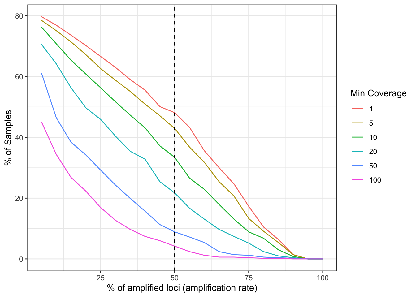

Figure 1: Sample success rate based on different thresholds of minimum read depth coverage per allele (ASV or amplicon sequence variant observed in the sample). x-axis represents the percentage of loci (amplicon or marker) which contains alleles that pass the threshold. y-axis represents the percentage of samples which amplify a specific percentage of loci given the allele detection threshold mentioned above. The plot represents all analyzed samples (no subsetting based on run and additional variables).

Let’s check the performance by sequencing run

ReadDepth_coverage = get_ReadDepth_coverage(ampseq_object_abd1, variable = 'Run')
  
sample_performance = ReadDepth_coverage$plot_read_depth_heatmap$data %>%
    mutate(Read_depth = case_when(
      is.na(Read_depth) ~ 0,
      !is.na(Read_depth) ~ Read_depth
    )) %>%
    summarise(amplified_amplicons1 = sum(Read_depth >= 1)/nrow(ampseq_object_abd1@markers),
              amplified_amplicons5 = sum(Read_depth >= 5)/nrow(ampseq_object_abd1@markers),
              amplified_amplicons10 = sum(Read_depth >= 10)/nrow(ampseq_object_abd1@markers),
              amplified_amplicons20 = sum(Read_depth >= 20)/nrow(ampseq_object_abd1@markers),
              amplified_amplicons50 = sum(Read_depth >= 50)/nrow(ampseq_object_abd1@markers),
              amplified_amplicons100 = sum(Read_depth >= 100)/nrow(ampseq_object_abd1@markers),
              Run = unique(var),
              .by = Sample_id) %>%
    pivot_longer(cols = starts_with('amplified_amplicons'), values_to = 'AmpRate', names_to = 'Threshold') %>%
    mutate(Threshold = as.integer(gsub('amplified_amplicons', '', Threshold)))

plot_precentage_of_samples_over_min_abd_byRun = sample_performance %>%
    summarise(AmpRate5 = round(100*sum(AmpRate >= .05)/n(), 1),
              AmpRate10 = round(100*sum(AmpRate >= .10)/n(), 1),
              AmpRate15 = round(100*sum(AmpRate >= .15)/n(), 1),
              AmpRate20 = round(100*sum(AmpRate >= .20)/n(), 1),
              AmpRate25 = round(100*sum(AmpRate >= .25)/n(), 1),
              AmpRate30 = round(100*sum(AmpRate >= .30)/n(), 1),
              AmpRate35 = round(100*sum(AmpRate >= .35)/n(), 1),
              AmpRate40 = round(100*sum(AmpRate >= .40)/n(), 1),
              AmpRate45 = round(100*sum(AmpRate >= .45)/n(), 1),
              AmpRate50 = round(100*sum(AmpRate >= .50)/n(), 1),
              AmpRate55 = round(100*sum(AmpRate >= .55)/n(), 1),
              AmpRate60 = round(100*sum(AmpRate >= .60)/n(), 1),
              AmpRate65 = round(100*sum(AmpRate >= .65)/n(), 1),
              AmpRate70 = round(100*sum(AmpRate >= .70)/n(), 1),
              AmpRate75 = round(100*sum(AmpRate >= .75)/n(), 1),
              AmpRate80 = round(100*sum(AmpRate >= .80)/n(), 1),
              AmpRate85 = round(100*sum(AmpRate >= .85)/n(), 1),
              AmpRate90 = round(100*sum(AmpRate >= .90)/n(), 1),
              AmpRate95 = round(100*sum(AmpRate >= .95)/n(), 1),
              AmpRate100 = round(100*sum(AmpRate >= 1)/n(), 1),
              .by = c(Threshold, Run)
    ) %>%
    pivot_longer(cols = paste0('AmpRate', seq(5, 100, 5)),
                 values_to = 'Percentage',
                 names_to = 'AmpRate') %>%
    mutate(AmpRate = as.numeric(gsub('AmpRate','', AmpRate)))%>%
    ggplot(aes(x = AmpRate, y = Percentage, color = as.factor(Threshold), group = as.factor(Threshold))) +
    geom_line() +
    geom_vline(xintercept = 50, linetype = 2) +
    facet_wrap(Run~., ncol = 3)+
    theme_bw() +
    labs(x = '% of amplified loci (amplification rate)', y = '% of Samples', color = 'Min Coverage')

plot_precentage_of_samples_over_min_abd_byRun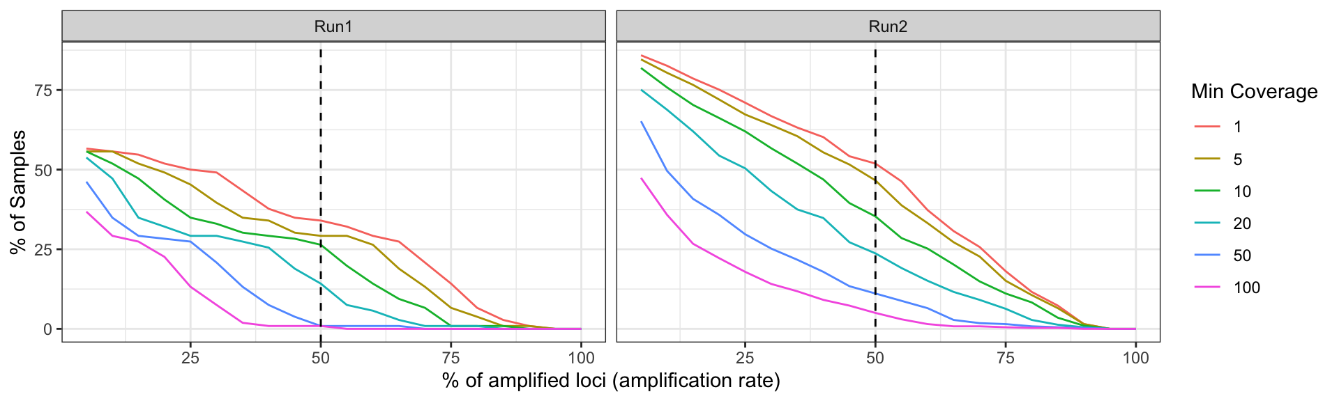

Figure 2: Sample success rate by Sequencing Run based on different thresholds of minimum read depth coverage per allele (ASV or amplicon sequence variant observed in the sample). x-axis represents the percentage of loci (amplicon or marker) which contains alleles that pass the threshold. y-axis represents the percentage of samples which amplify a specific percentage of loci given the allele detection threshold mentioned above.

Let’s do it by Country

ReadDepth_coverage = get_ReadDepth_coverage(ampseq_object_abd1, variable = 'Country')

sample_performance = ReadDepth_coverage$plot_read_depth_heatmap$data %>%
      filter(!is.na(var))%>%
      mutate(Read_depth = case_when(
        is.na(Read_depth) ~ 0,
        !is.na(Read_depth) ~ Read_depth
      )) %>%
      summarise(amplified_amplicons1 = sum(Read_depth >= 1)/nrow(ampseq_object_abd1@markers),
                amplified_amplicons5 = sum(Read_depth >= 5)/nrow(ampseq_object_abd1@markers),
                amplified_amplicons10 = sum(Read_depth >= 10)/nrow(ampseq_object_abd1@markers),
                amplified_amplicons20 = sum(Read_depth >= 20)/nrow(ampseq_object_abd1@markers),
                amplified_amplicons50 = sum(Read_depth >= 50)/nrow(ampseq_object_abd1@markers),
                amplified_amplicons100 = sum(Read_depth >= 100)/nrow(ampseq_object_abd1@markers),
                Country = unique(var),
                .by = Sample_id) %>%
      pivot_longer(cols = starts_with('amplified_amplicons'), values_to = 'AmpRate', names_to = 'Threshold') %>%
      mutate(Threshold = as.integer(gsub('amplified_amplicons', '', Threshold)))

plot_precentage_of_samples_over_min_abd_byCountry = sample_performance %>%
      summarise(AmpRate5 = round(100*sum(AmpRate >= .05)/n(), 1),
                AmpRate10 = round(100*sum(AmpRate >= .10)/n(), 1),
                AmpRate15 = round(100*sum(AmpRate >= .15)/n(), 1),
                AmpRate20 = round(100*sum(AmpRate >= .20)/n(), 1),
                AmpRate25 = round(100*sum(AmpRate >= .25)/n(), 1),
                AmpRate30 = round(100*sum(AmpRate >= .30)/n(), 1),
                AmpRate35 = round(100*sum(AmpRate >= .35)/n(), 1),
                AmpRate40 = round(100*sum(AmpRate >= .40)/n(), 1),
                AmpRate45 = round(100*sum(AmpRate >= .45)/n(), 1),
                AmpRate50 = round(100*sum(AmpRate >= .50)/n(), 1),
                AmpRate55 = round(100*sum(AmpRate >= .55)/n(), 1),
                AmpRate60 = round(100*sum(AmpRate >= .60)/n(), 1),
                AmpRate65 = round(100*sum(AmpRate >= .65)/n(), 1),
                AmpRate70 = round(100*sum(AmpRate >= .70)/n(), 1),
                AmpRate75 = round(100*sum(AmpRate >= .75)/n(), 1),
                AmpRate80 = round(100*sum(AmpRate >= .80)/n(), 1),
                AmpRate85 = round(100*sum(AmpRate >= .85)/n(), 1),
                AmpRate90 = round(100*sum(AmpRate >= .90)/n(), 1),
                AmpRate95 = round(100*sum(AmpRate >= .95)/n(), 1),
                AmpRate100 = round(100*sum(AmpRate >= 1)/n(), 1),
                .by = c(Threshold, Country)
      ) %>%
      pivot_longer(cols = paste0('AmpRate', seq(5, 100, 5)),
                   values_to = 'Percentage',
                   names_to = 'AmpRate') %>%
      mutate(AmpRate = as.numeric(gsub('AmpRate','', AmpRate)))%>%
      ggplot(aes(x = AmpRate, y = Percentage, color = as.factor(Threshold), group = as.factor(Threshold))) +
      geom_line() +
      geom_vline(xintercept = 50, linetype = 2) +
      facet_wrap(Country~., ncol = 3)+
      theme_bw() +
      labs(x = '% of amplified loci (amplification rate)', y = '% of Samples', color = 'Min Coverage')

plot_precentage_of_samples_over_min_abd_byCountry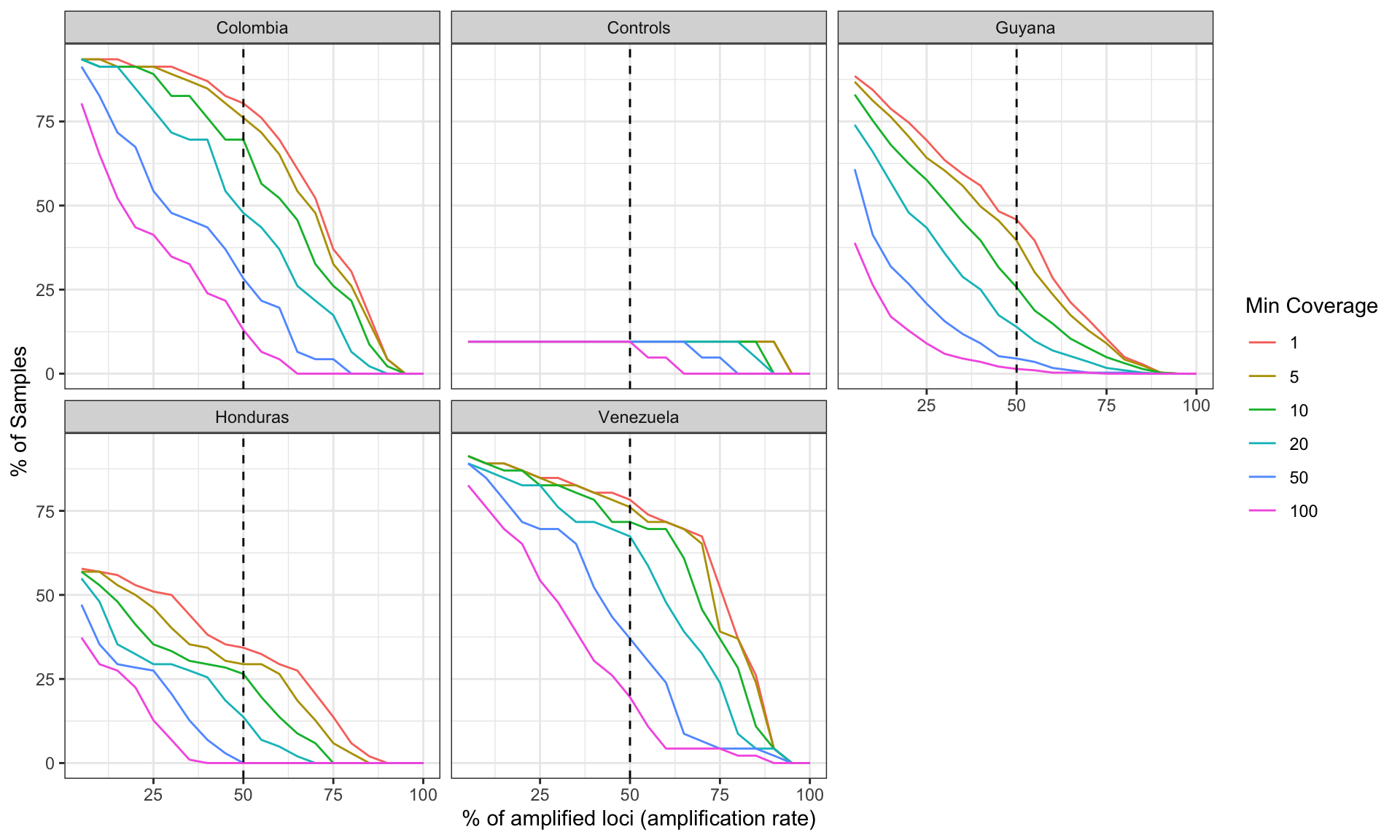

Figure 3: Sample success rate by Sequencing Run based on different thresholds of minimum read depth coverage per allele (ASV or amplicon sequence variant observed in the sample). x-axis represents the percentage of loci (amplicon or marker) which contains alleles that pass the threshold. y-axis represents the percentage of samples which amplify a specific percentage of loci given the allele detection threshold mentioned above.

Identifying likely genotyping errors

After the denoising process of the fastq files, the cigar table might contains some artefacts that affect downstream analysis. These artifacts include systematic PCR errors (off-target products and stutters in INDELs) as well as stochastic PCR errors. All these artifacts coexist with the true allele within the sample, causing the observation of two or more alleles (the true allele plus the artifacts) in the particular loci of the sample where the error has occurred, the increment of the heterozygousity of the loci (if the error is systematic), and the increment of polyclonal infections in the population.

However, when analyzing a population we do not expect all samples to be polyclonal, and it should not be possible to find a locus that is heterozygous for all samples. Moreover, loci with alternative alleles only present in heterozygous samples should be rare as they are the result of “de-novo” mutations, and the frequency of heterozygous samples for that loci should be low because samples comes from different regions and we do not expect a wide geographic distribution of that genotype (This might not be true if only one population is been analyzed).

Here the identification and removal of likely genotyping errors is done in three sequential steps: 1) Removal of off-target products, 2) masking of INDELs present in flanking regions of the ASV, 3) and removal of stochastic PCR errors (alleles mainly present as minor alleles).

The identification of all these likely genotyping errors is based on the following parameters:

dVSITES_ij: Density of variant sites (SNPs and INDELs) in the allele (ASV) \(j\) of the locus \(i\).
P_ij (\(P_{i,j}\)): The total number of samples that amplified each alternative allele \(j\) in locus \(i\).
H_ij (\(H_{i,j}\)): Number of heterozygous samples in the locus \(i\) that carry the alternative allele \(j\).
H_ijminor (\(H_{i,jminor}\)): Number of heterozygous samples in the locus \(i\) where the alternative allele \(j\) is the minor Allele (the allele with the lower read counts).
h_ij (\(h_{i,j}=H_{i,j}/P_{i,j}\)): ratio of heterozygous samples in the locus that carry the alternative allele of interest respect to the total number of samples that amplified alternative allele.
h_ijminor (\(h_{i,jminor}=H_{i,jminor}/H_{i,j}\)): ratio of heterozygous samples where the alternative allele is the minor Allele respect to the total number of heterozygous samples in the locus that carry the alternative allele.
p_ij (\(p_{i,j}\)): population prevalence of the alternative allele \(j\) in locus \(i\).
flanking_INDEL: Boolean that specify if there are INDELs in the flanking region of the ASV.
SNV_in_homopolymer: Boolean that specify if there are SNVs in an homopolymer region. By default and homopolymer is defined as a region of a single nucleotide repeated 5 times in tandem.
INDEL_in_homopolymer: Boolean that specify if there are SNVs in an homopolymer region. By default and homopolymer is defined as a region of a single nucleotide repeated 5 times in tandem.

One of the consequences of the geontyping erros, is the increment of heterozygousity in the loci where those errors occurs. Lets check the distribution of the observed heterozygosity by locus, and the distribution of other metrics of the alternative alleles.

ref_fasta = '~/Documents/Github/MHap-Analysis/docs/reference/Pviv_P01/PvGTSeq271_refseqs.fasta'

Alt_ASVs_stats = 
  get_ASVs_attributes(ampseq_object, 
                      ref_fasta = ref_fasta)

h_ij_thres = 0.5
h_ijminor_thres = 0.5
Hetob_j_thres = 0.05


plot_Hetob_j = Alt_ASVs_stats %>%
  ggplot(aes(x= Hetob_j)) + 
    geom_vline(xintercept = Hetob_j_thres,
               linetype = 2) +
    geom_histogram(binwidth = 0.01) + 
    theme_bw()

plot_h_ij = Alt_ASVs_stats %>%
  ggplot(aes(x= h_ij)) + 
    geom_vline(xintercept = h_ij_thres,
               linetype = 2) +
    geom_histogram(binwidth = 0.01) + 
    theme_bw()

plot_h_ijminor = Alt_ASVs_stats %>%
  ggplot(aes(x= h_ijminor)) + 
    geom_vline(xintercept = h_ijminor_thres,
               linetype = 2) +
    geom_histogram(binwidth = 0.01) + 
    theme_bw()

Alt_ASVs_metrics_distribution = Alt_ASVs_stats %>%
  mutate(h_ijminor_cat = case_when(
        h_ijminor < h_ijminor_thres ~ paste0('h_ijminor < ',h_ijminor_thres),
        h_ijminor >= h_ijminor_thres ~ paste0('h_ijminor >= ',h_ijminor_thres)),
        
      Hetob_j_cat = case_when(
        Hetob_j < Hetob_j_thres ~ paste0('Hetob_j < ',Hetob_j_thres),
        Hetob_j >= Hetob_j_thres ~ paste0('Hetob_j >= ',Hetob_j_thres)
      )
        
        )%>%
      ggplot(aes(x = p_ij, 
                 y = h_ij,
                 color = h_ijminor,
                 size = Hetob_j))+
      geom_point()+
      geom_hline(yintercept = h_ij_thres,
                 linetype = 2) +
      theme_bw()+
      scale_color_continuous(type = 'viridis')+
      facet_grid(Hetob_j_cat ~ h_ijminor_cat)+
      labs(x = 'Alternative allele prev. (p_ij)',
           y = 'h_ij (H_ij/P_ij)',
           color = 'h_ijminor')

Alt_ASVs_metrics_distribution = ggdraw()+
  draw_plot(plot_Hetob_j, 
                x = 0, width = .4,
                y = 0.66, height = .34)+
  draw_plot(plot_h_ij, 
                x = 0, width = .4,
                y = 0.33, height = .33)+
  draw_plot(plot_h_ijminor, 
                x = 0, width = .4,
                y = 0, height = .33)+
  draw_plot(Alt_ASVs_metrics_distribution, 
                x = .4, width = .6,
                y = 0, height = 1)
      
Alt_ASVs_metrics_distribution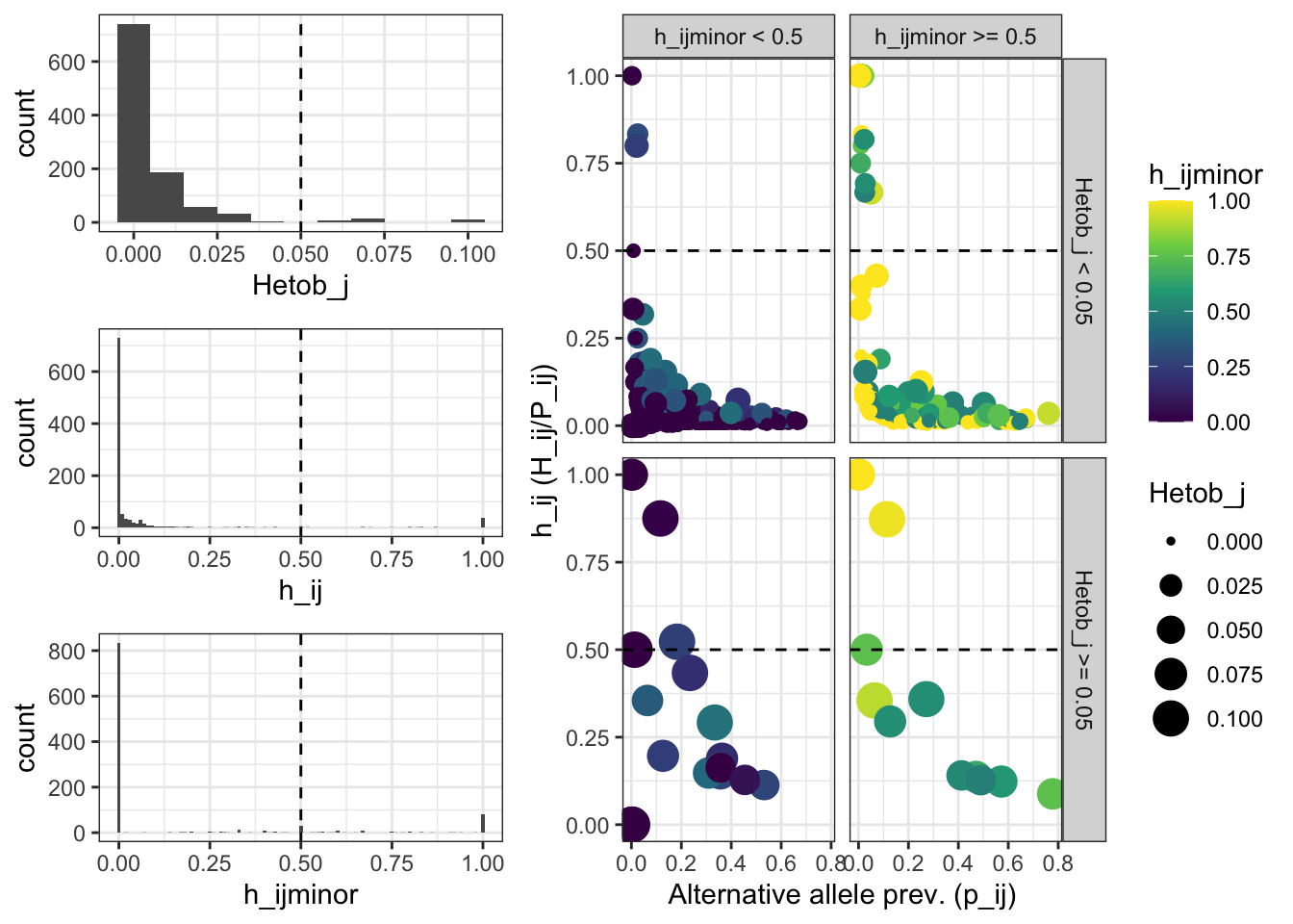

Identification and removal of off-target products

A non-specific product is the result of the amplification of a DNA template that shares a certain degree of identity in the region of the primers with the desired target. However, the degree of identity of these off-targets with respect to the desired target tends to be low, generating a high density of polymorphisms in the alignment between the off-target ASV and the reference template. For that reason in this step we use the density of of variant sites (dVSITES_ij) in order to identify alleles that are potentially off-target products. The other parameters explained above can also be included to constraint more the definition. The filtering criteria can be specified with the argument “mask_formula” (maskt_formula = "dVSITES_ij >= 0.3").

Run the function get_ASVs_attributes:

off_target_stats = get_ASVs_attributes(ampseq_object, 
                                       ref_fasta = ref_fasta)

Generate a histogram of the density of variant sites per allele.

dVSITES_ij_thres = 0.25

plot_off_target_stats = off_target_stats %>%
    ggplot(aes(x= dVSITES_ij)) + 
    geom_vline(xintercept = dVSITES_ij_thres,
               linetype = 2) +
    geom_histogram(binwidth = 0.01) + 
    theme_bw()

plot_off_target_stats2 = off_target_stats %>%
      mutate(h_ijminor_cat = case_when(
        h_ijminor < h_ijminor_thres ~ paste0('h_ijminor < ',h_ijminor_thres),
        h_ijminor >= h_ijminor_thres ~ paste0('h_ijminor >= ',h_ijminor_thres)
      ),
      dVSITES_ij_cat = case_when(
        dVSITES_ij >= dVSITES_ij_thres ~ 'dVSITES_ij >= 0.25',
        dVSITES_ij < dVSITES_ij_thres ~ 'dVSITES_ij < 0.25'
      ),
      Hetob_j_cat = case_when(
        Hetob_j < Hetob_j_thres ~ paste0('Hetob_j < ',Hetob_j_thres),
        Hetob_j >= Hetob_j_thres ~ paste0('Hetob_j >= ',Hetob_j_thres)
      )
      )%>%
      ggplot(aes(x = p_ij, 
                 y = h_ij,
                 color = h_ijminor,
                 size = dVSITES_ij))+
      geom_point()+
      geom_hline(yintercept = h_ij_thres,
                 linetype = 2) +
      theme_bw()+
      scale_color_continuous(type = 'viridis')+
      facet_grid(dVSITES_ij_cat ~ Hetob_j_cat + h_ijminor_cat)+
      labs(x = 'Alternative allele prev. (p_ij)',
           y = 'h_ij (H_ij/P_ij)',
           color = 'h_ijminor')
    
    plot_off_target_stats = ggdraw()+
      draw_plot(plot_off_target_stats, 
                x = 0, width = .4,
                y = 0, height = 1)+
      draw_plot(plot_off_target_stats2, 
                x = .4, width = .6,
                y = 0, height = 1)

plot_off_target_stats

Figure 4: Identifcation of off-target products. Histogram represents the distribution of the densitity of variant sites in each allele in each locus (dVSITES_ij). The scatter plot shows the distribution of the prevalence of the alternative allele (p_ij), the frequency of the alternative allele as heterozygous (h_ij), the frequency of the alternative allele as minor allele (h_ijminor), and the density of variant sites (dVSITES_ij) of the alternative allele respect to the reference template.

Identify how many alleles would be removed using a filter of 0.25.

n_off_target_alleles = off_target_stats[off_target_stats$dVSITES_ij >= dVSITES_ij_thres,][['Allele']]

print(paste0(length(n_off_target_alleles), ' allele(s) match(es) the criteria to define off-target products'))

## [1] "22 allele(s) match(es) the criteria to define off-target products"

Check what are those allele:

View(off_target_stats%>%
  filter(dVSITES_ij >= dVSITES_ij_thres))

remove off-target products:

ampseq_object = mask_alt_alleles(ampseq_object, mask_formula = 'dVSITES_ij >= 0.25', ref_fasta = ref_fasta)

## [1] "Filter dVSITES_ij >= 0.25 will be applied"

Products with flanking INDELs

Flanking INDELs are defined as INDELs that occurs at the beginning or the end of the ASV attached to the primer area. Flanking INDELs can lead to primer miss binding during PCR by creating additional alleles which differs in the length of the INDEL in the same sample. The filtering criteria can be specified in Terra with the argument “flanking_INDEL_formula” (by default "flanking_INDEL_formula": "flanking_INDEL==TRUE&h_ij>=0.66").

Identified Flanking INDELs are masked, which means the the internal region of the ASV is kept to define the allele.

Run the function again get_ASVs_attributes:

flanking_INDEL_stats = get_ASVs_attributes(ampseq_object, 
                                            ref_fasta = ref_fasta)

Generate a scatter plot of the density of variant sites per allele.

plot_flanking_INDEL_stats = flanking_INDEL_stats %>%
      mutate(h_ijminor_cat = case_when(
        h_ijminor < h_ijminor_thres ~ paste0('h_ijminor < ',h_ijminor_thres),
        h_ijminor >= h_ijminor_thres ~ paste0('h_ijminor >= ',h_ijminor_thres)),
        flanking_INDEL_cat = case_when(
        flanking_INDEL == TRUE ~ 'w/. flanking INDELs',
        flanking_INDEL == FALSE ~ 'w/o flanking INDELs'
      ),
      Hetob_j_cat = case_when(
        Hetob_j < Hetob_j_thres ~ paste0('Hetob_j < ',Hetob_j_thres),
        Hetob_j >= Hetob_j_thres ~ paste0('Hetob_j >= ',Hetob_j_thres)
      )
        
        )%>%
      ggplot(aes(x = p_ij, 
                 y = h_ij,
                 color = h_ijminor,
                 size = Hetob_j))+
      geom_point()+
      geom_hline(yintercept = h_ij_thres,
                 linetype = 2) +
      theme_bw()+
      scale_color_continuous(type = 'viridis')+
      facet_grid(flanking_INDEL_cat ~ Hetob_j_cat + h_ijminor_cat)+
      labs(x = 'Alternative allele prev. (p_ij)',
           y = 'h_ij (H_ij/P_ij)',
           color = 'h_ijminor')

plot_flanking_INDEL_stats

Figure 5: Identification of flanking INDELs. The scatter plot shows the distribution of the prevalence of the alternative allele (p_ij), the frequency of the alternative allele as heterozygous (h_ij), and the frequency of the alternative allele as minor allele (h_ijminor). The panels FALSE and TRUE represent alleles that do not contain or contain flanking INDELs.

Identify how many alleles would be removed using flanking_INDEL == TRUE:

n_flanking_INDEL_alleles = flanking_INDEL_stats[flanking_INDEL_stats$flanking_INDEL == TRUE, ][['Allele']]
print(paste0(length(n_flanking_INDEL_alleles), ' allele(s) match(es) the criteria to identify products with flanking INDELs'))

## [1] "21 allele(s) match(es) the criteria to identify products with flanking INDELs"

View(
  flanking_INDEL_stats %>%
    filter(flanking_INDEL == TRUE)
)

Mask alleles with flanking indels:

while(length(n_flanking_INDEL_alleles) > 0){
  ampseq_object = mask_alt_alleles(ampseq_object, mask_formula = 'flanking_INDEL == TRUE',
                                      ref_fasta = ref_fasta)
  
  flanking_INDEL_stats2 = get_ASVs_attributes(ampseq_object, 
                                            ref_fasta = ref_fasta)
  n_flanking_INDEL_alleles = 
    flanking_INDEL_stats2[flanking_INDEL_stats2$flanking_INDEL == TRUE, ][['Allele']]
}

## [1] "Filter flanking_INDEL == TRUE will be applied"

PCR errors due to homopolymers

Run the function again get_ASVs_attributes:

homopolymers_stats = get_ASVs_attributes(ampseq_object, 
                                            ref_fasta = ref_fasta)

Generate a scatter plot of the density of variant sites per allele.

plot_homopolymers_stats = homopolymers_stats %>%
      mutate(h_ijminor_cat = case_when(
        h_ijminor < h_ijminor_thres ~ paste0('h_ijminor < ',h_ijminor_thres),
        h_ijminor >= h_ijminor_thres ~ paste0('h_ijminor >= ',h_ijminor_thres)
      ),
      
      vsites_in_homopopylmers = case_when(
        SNV_in_homopolymer == FALSE & INDEL_in_homopolymer == FALSE ~ 'No VSites in Hom.',
        SNV_in_homopolymer == TRUE ~ 'SNV in Hom.',
        INDEL_in_homopolymer == TRUE ~ 'INDEL in Hom.'
      ),
      
      vsites_in_homopopylmers = factor(vsites_in_homopopylmers,
                                       levels = c('No VSites in Hom.',
                                                  'SNV in Hom.',
                                                  'INDEL in Hom.')),
      Hetob_j_cat = case_when(
        Hetob_j < Hetob_j_thres ~ paste0('Hetob_j < ',Hetob_j_thres),
        Hetob_j >= Hetob_j_thres ~ paste0('Hetob_j >= ',Hetob_j_thres)
      )
      
      )%>%
      ggplot(aes(x = p_ij, 
                 y = h_ij,
                 color = h_ijminor,
                 size = Hetob_j))+
      geom_point()+
      geom_hline(yintercept = h_ij_thres,
                 linetype = 2) +
      theme_bw()+
      scale_color_continuous(type = 'viridis')+
      facet_grid(vsites_in_homopopylmers ~ Hetob_j_cat + h_ijminor_cat )+
      labs(x = 'Alternative allele prev. (p_ij)',
           y = 'h_ij (H_ij/P_ij)',
           color = 'h_ijminor')

plot_homopolymers_stats

Identify how many alleles would be removed using SNV_in_homopolymer == TRUE:

n_snv_in_homopolymer_alleles = homopolymers_stats[
  homopolymers_stats$SNV_in_homopolymer == TRUE & 
    (homopolymers_stats$h_ij > h_ij_thres & homopolymers_stats$h_ijminor > h_ijminor_thres ), ][['Allele']]
print(paste0(length(n_snv_in_homopolymer_alleles), ' allele(s) match(es) the criteria to identify products with SNVs in homopolymers'))

## [1] "3 allele(s) match(es) the criteria to identify products with SNVs in homopolymers"

Identify how many alleles would be removed using INDEL_in_homopolymer == TRUE:

n_indel_in_homopolymer_alleles = homopolymers_stats[homopolymers_stats$INDEL_in_homopolymer == TRUE &
                                                      homopolymers_stats$h_ij > h_ij_thres, ][['Allele']]
print(paste0(length(n_indel_in_homopolymer_alleles), ' allele(s) match(es) the criteria to identify products with INDELs in homopolymers'))

## [1] "1 allele(s) match(es) the criteria to identify products with INDELs in homopolymers"

Mask alleles with SNVs or INDELs in homopolymers

ampseq_object = mask_alt_alleles(
  ampseq_object, 
  mask_formula = '(SNV_in_homopolymer == TRUE | INDEL_in_homopolymer == TRUE) & h_ij >= 0.5 & h_ijminor >= 0.5', 
  ref_fasta = ref_fasta)

## [1] "Filter SNV_in_homopolymer == TRUE will be applied"
## [1] "Filter INDEL_in_homopolymer == TRUE will be applied"
## [1] "Filter h_ij >= 0.5 will be applied"
## [1] "Filter h_ijminor >= 0.5 will be applied"

Stochastic PCR errors

PCR errors introduce new alleles in both polymorphic and monomorphic sites. These errors depend on the error rate of the polymerases used in the sWGA and library generation steps, and they will generate alternative alleles that are mainly present as the minor allele at a heterozygous site and their frequency tends to be low in the population. By analyzing the distribution of population frequency of each alternative allele p_ij (\(p_{i,j}\)), the ratio of heterozygous samples in the locus that carry the alternative allele of interest respect to the total number of samples that amplified alternative allele h_ij (\(h_{i,j}\)), and the ratio of heterozygous samples where the alternative allele is the minor allele respect to the total number of heterozygous samples h_ijminor (\(h_{i,jminor}\)), in this step we will remove all alternative alleles that match our filtering criteria. This filtering criteria can be specified in Terra with the argument “PCR_errors_formula” (by default “PCR_errors_formula”: "h_ij>=0.66&h_ijminor>= 0.66")

Use again the function get_ASVs_attributes

PCR_errors_stats = get_ASVs_attributes(ampseq_object, ref_fasta = ref_fasta)

Use an scatter plot to visualize alleles about the thresholds.

plot_PCR_errors_stats = PCR_errors_stats %>%
      mutate(h_ijminor_cat = case_when(
        h_ijminor < h_ijminor_thres ~ paste0('h_ijminor < ',h_ijminor_thres),
        h_ijminor >= h_ijminor_thres ~ paste0('h_ijminor >= ',h_ijminor_thres)
      ),
      Hetob_j_cat = case_when(
        Hetob_j < Hetob_j_thres ~ paste0('Hetob_j < ',Hetob_j_thres),
        Hetob_j >= Hetob_j_thres ~ paste0('Hetob_j >= ',Hetob_j_thres))
      )%>%
      ggplot(aes(x = p_ij, 
                 y = h_ij,
                 color = h_ijminor,
                 size = Hetob_j))+
      geom_point()+
      geom_hline(yintercept = h_ij_thres,
                 linetype = 2) +
      theme_bw()+
      scale_color_continuous(type = 'viridis')+
      facet_grid(Hetob_j_cat~h_ijminor_cat)+
      labs(x = 'Alternative allele prev. (p_ij)',
           y = 'h_ij (H_ij/P_ij)',
           color = 'h_ijminor')

plot_PCR_errors_stats

Figure 6: Identification and removal of stochastic PCR errors. The scatter plot shows the distribution of the prevalence of the alternative allele (p_ij), the frequency of the alternative allele as heterozygous (h_ij), and the frequency of the alternative allele as minor allele (h_ijminor). The horizontal panels are defined based on the threshold stablished for h_ijminor.

How many alleles didn’t pass the threshold

n_PCR_errors_alleles = PCR_errors_stats[PCR_errors_stats$h_ij >= 0.66 & PCR_errors_stats$h_ijminor >= 0.66, ][['Allele']]
print(paste0(length(n_PCR_errors_alleles), ' allele(s) match(es) the criteria to identify PCR_errors'))

## [1] "16 allele(s) match(es) the criteria to identify PCR_errors"

View(
  PCR_errors_stats %>%
    filter(h_ij >= 0.66 & h_ijminor >= 0.66))

Remove stochastic PCR errors:

ampseq_object = mask_alt_alleles(
  ampseq_object, 
  mask_formula = 'h_ij >= 0.5 & h_ijminor >= 0.5', 
  ref_fasta = ref_fasta)

## [1] "Filter h_ij >= 0.5 will be applied"
## [1] "Filter h_ijminor >= 0.5 will be applied"

After removing and masking suspicious alleles, the distribution of the different metrics looks as follows:

Alt_ASVs_stats = 
  get_ASVs_attributes(ampseq_object, 
                      ref_fasta = ref_fasta)

plot_Hetob_j = Alt_ASVs_stats %>%
  ggplot(aes(x= Hetob_j)) + 
    geom_vline(xintercept = Hetob_j_thres,
               linetype = 2) +
    geom_histogram(binwidth = 0.01) + 
    theme_bw()

plot_h_ij = Alt_ASVs_stats %>%
  ggplot(aes(x= h_ij)) + 
    geom_vline(xintercept = h_ij_thres,
               linetype = 2) +
    geom_histogram(binwidth = 0.01) + 
    theme_bw()

plot_h_ijminor = Alt_ASVs_stats %>%
  ggplot(aes(x= h_ijminor)) + 
    geom_vline(xintercept = h_ijminor_thres,
               linetype = 2) +
    geom_histogram(binwidth = 0.01) + 
    theme_bw()

Alt_ASVs_metrics_distribution = Alt_ASVs_stats %>%
  mutate(h_ijminor_cat = case_when(
        h_ijminor < h_ijminor_thres ~ paste0('h_ijminor < ',h_ijminor_thres),
        h_ijminor >= h_ijminor_thres ~ paste0('h_ijminor >= ',h_ijminor_thres)),
        
      Hetob_j_cat = case_when(
        Hetob_j < Hetob_j_thres ~ paste0('Hetob_j < ',Hetob_j_thres),
        Hetob_j >= Hetob_j_thres ~ paste0('Hetob_j >= ',Hetob_j_thres)
      )
        
        )%>%
      ggplot(aes(x = p_ij, 
                 y = h_ij,
                 color = h_ijminor,
                 size = Hetob_j))+
      geom_point()+
      geom_hline(yintercept = h_ij_thres,
                 linetype = 2) +
      theme_bw()+
      scale_color_continuous(type = 'viridis')+
      facet_grid(Hetob_j_cat~h_ijminor_cat)+
      labs(x = 'Alternative allele prev. (p_ij)',
           y = 'h_ij (H_ij/P_ij)',
           color = 'h_ijminor')

Alt_ASVs_metrics_distribution = ggdraw()+
  draw_plot(plot_Hetob_j, 
                x = 0, width = .4,
                y = 0.66, height = .34)+
  draw_plot(plot_h_ij, 
                x = 0, width = .4,
                y = 0.33, height = .33)+
  draw_plot(plot_h_ijminor, 
                x = 0, width = .4,
                y = 0, height = .33)+
  draw_plot(Alt_ASVs_metrics_distribution, 
                x = .4, width = .6,
                y = 0, height = 1)
      
Alt_ASVs_metrics_distribution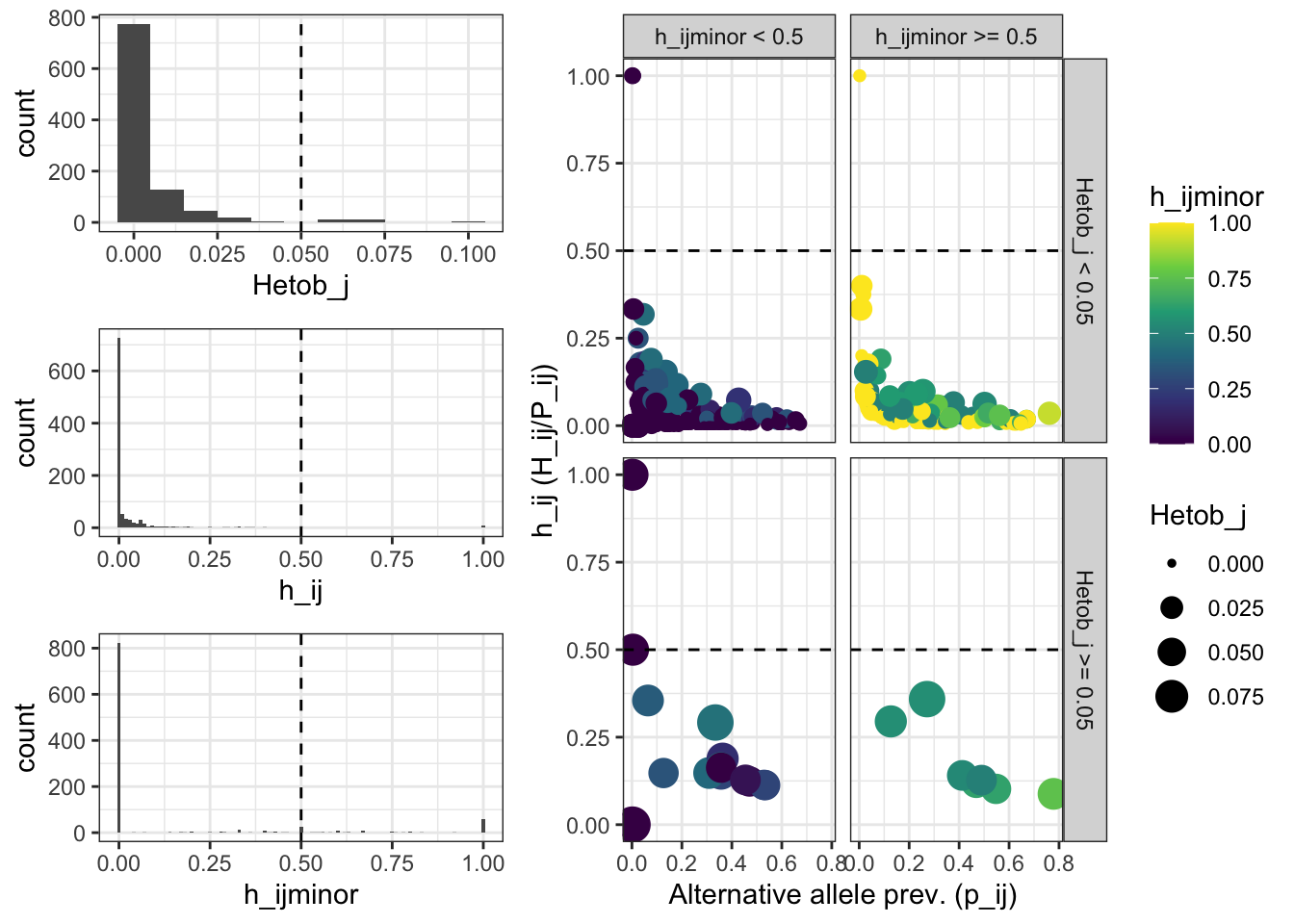

Read depth yield per sample and locus

Inspect again the read depth coverage of our data:

ReadDepth_coverage = get_ReadDepth_coverage(ampseq_object, variable = 'Country')

ReadDepth_coverage$plot_read_depth_heatmap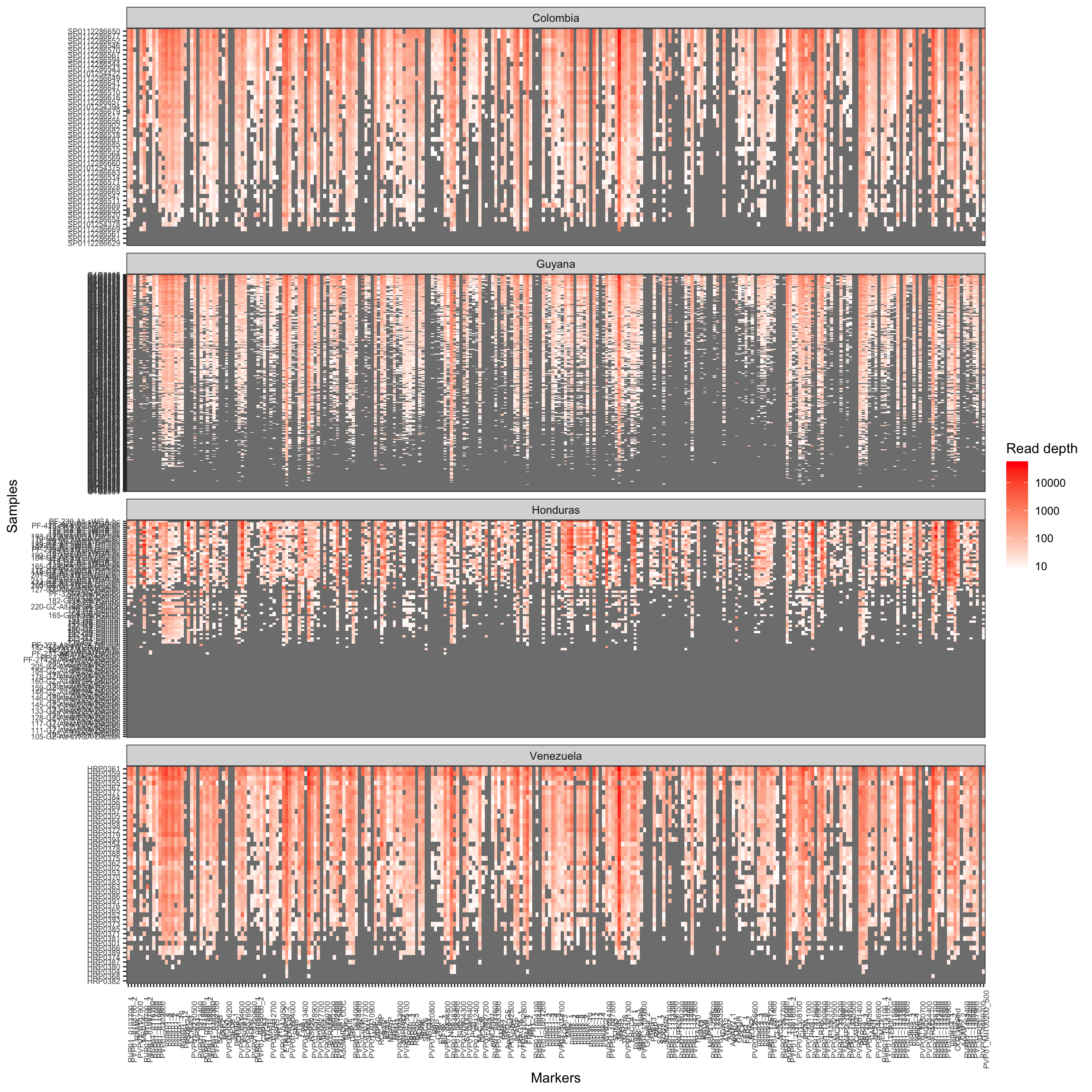

Figure 7: Read Coverage per sample per locus. The heatmaps show the number of read-pairs obtained per sample (rows) at each locus (columns). Separate panels are used for each value of Variable1 (e.g., sample geographic origin). Darker reds indicate higher read-depth. Grey indicates lack of signal for the locus/sample.

Retention of loci and samples for subsequent analysis

Locus performance across different countries

all_loci_amplification_rate = locus_amplification_rate(ampseq_object, threshold = 0.65, strata = 'Country', update_loci = F)

fig8.height = 2*length(unique(all_loci_amplification_rate$data$Strata))

all_loci_amplification_rate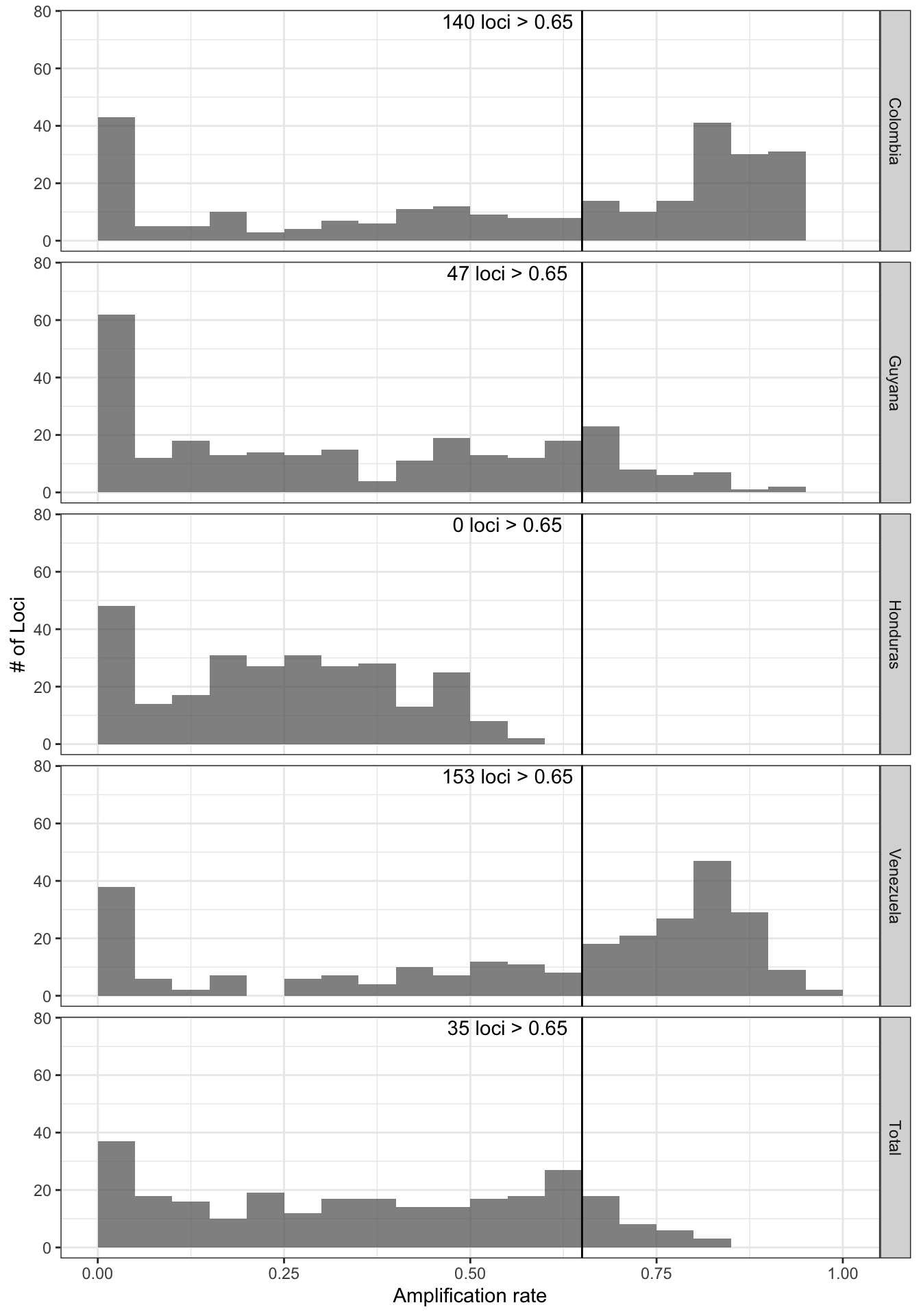

Figure 10: Locus amplification rate distribution across categories in Variable1. Each panel represents the cateories of Variable1, and the bottom panel represents the total population and the actual number of loci that are retained. Vertical line represents the locus_ampl_rate threshold set by the user.

Keep loci with more than 50% of amplified samples in at least one of the countries:

ampseq_object = locus_amplification_rate(ampseq_object, threshold = 0.5, strata = 'Country', update_loci = T, based_on_strata = T)

Retention of samples for subsequent analysis

Use the function sample_amplification_rate:

samples_amplification_rate = sample_amplification_rate(ampseq_object, threshold = 0.8, strata = 'Country', update_samples = F)

fig9.height = 2*length(unique(samples_amplification_rate$data$Strata))

samples_amplification_rate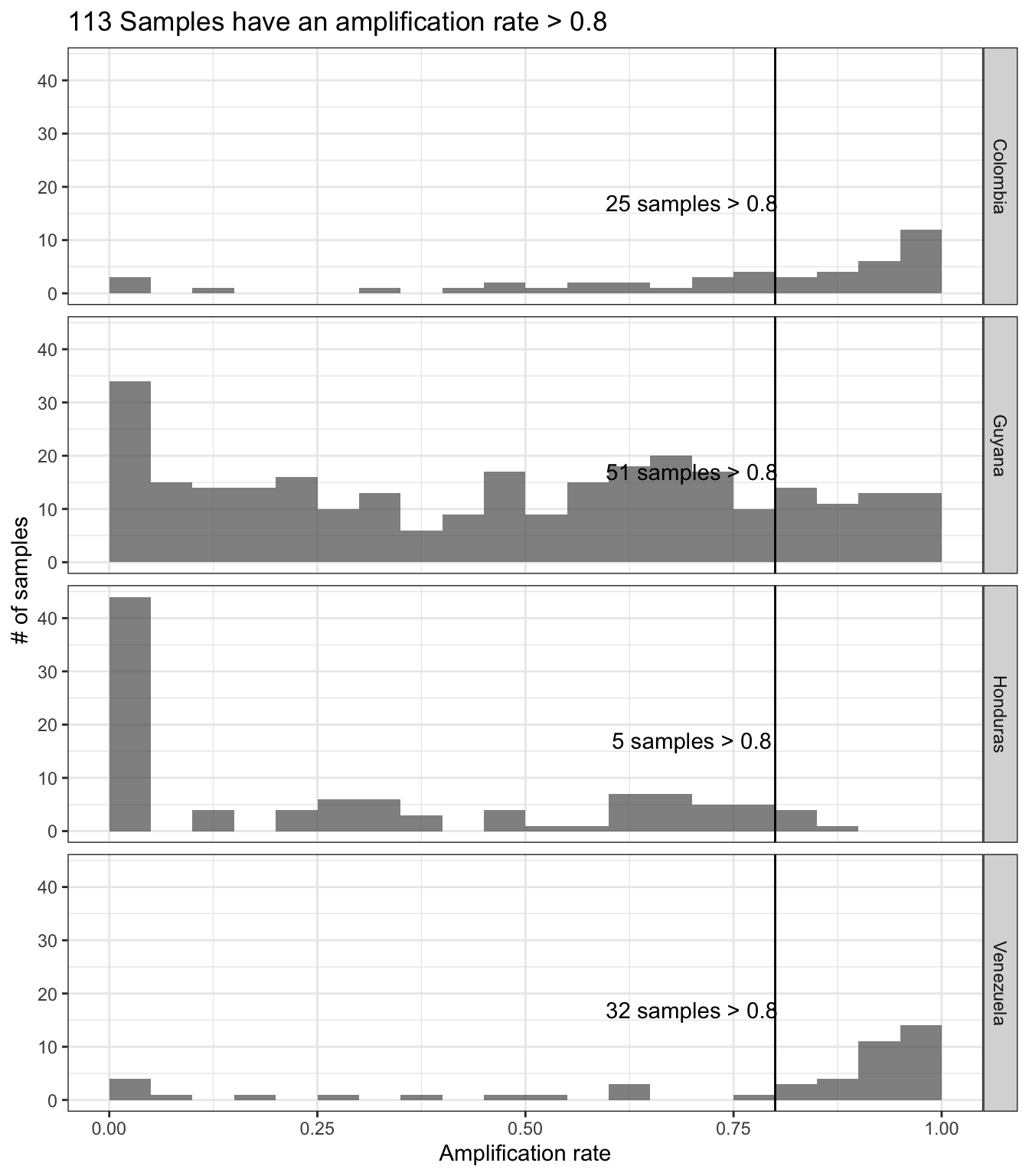

Figure 11: Sample amplification rate distribution across categories in Variable1. Each panel represents the categories of Variable1 and the number within each panel represents the number of samples that are retained in each category.

Keep samples with at least 50% of amplified loci

ampseq_object = sample_amplification_rate(ampseq_object, threshold = 0.5, strata = 'Country', update_samples = T)

Export the filtered ampseq_object

As Excel file

write_ampseq(ampseq_object, name = '~/Documents/Github/MHap-Analysis/docs/data/Pviv_example/Pviv_ampseq_filtered.xlsx', format = 'excel')

The exported ampseq object can also be uploaded in R to be used for other pipelines

ampseq_object2 = read_ampseq(file = '~/Documents/Github/MHap-Analysis/docs/data/Pviv_example/Pviv_ampseq_filtered.xlsx', 
                   format = 'excel')

As csv files

write_ampseq(ampseq_object, name = '~/Documents/Github/MHap-Analysis/docs/data/Pviv_example/Pviv_ampseq_filtered', format = 'csv')