PvGTSeq: a targeted amplicon sequencing for Plasmodium vivax
Neafsey Lab
The purpose of this tutorial is give insight on the bioinformatic analysis of the PvGTSeq panel. This tutorial will cover:
Denoising fastq files through the Dada2 based pipeline.
Aligning ASVs to reference genome and summarizing the haplotype information in Pseudo-CIGAR format.
Importing and handling tables in CIGAR format in R environment.
Molecular surveillance of drug resistance.
Genetic subdivision
Dada2 based pipeline: malaria-amplicon-pipeline
This pipeline is based on Dada2 R Package. For more documentation and tutorials about Dada2 and its functionalities please look a the following links:
- https://benjjneb.github.io/dada2/
- https://bioconductor.org/packages/devel/bioc/vignettes/dada2/inst/doc/dada2-intro.html
- https://benjjneb.github.io/dada2/tutorial.html
- https://benjjneb.github.io/dada2/tutorial_1_8.html
The documentation of this pipeline is here. Before to start you will require to install Anaconda 3, and download and create the ampseq enviroment.
Denoising fastq files:
On the terminal, use the environment.yml file (or the
environment_mac.yml for macos system) to create a conda
virtual environment:
conda env create --file environment.yml -p /path/to/env/<name-of-environment>/To activate the conda environment write the following line in the terminal:
source activate <name-of-environment>All inputs (files and specifications on how to run the pipeline)
should be provided using a .json file.
Apart of the fastq files, there are three input files that are required to run the pipeline:
PvGTSeq271_fwd.fasta: Fasta file with the sequence of the forward primers without including the adapters.PvGTSeq271_rvs.fasta: Fasta file with the sequence of the reverse primers without including the adapters.
Additional you require to generate a .csv file, called
metafile.csv (you can name it as you want) with the path to
all the fastq files. You can use the scripts create_meta.R
or create_meta.py to generate that file.
Your .json file should looks like this:
{
  "##_COMMENT_##": "INPUTS",
  "tool": "",
  "run_dir": "",
  "path_to_meta": "PATHS_TO/PvGTSeq_metafile.csv",
  "preprocess": 1,
  "remove_primer": 1,
  "Class": "parasite",
  "dada2_default": 0,
  "maxEE": "5,5",
  "trimRight": "2,2",
  "minLen": 30,
  "truncQ": "5,5",
  "max_consist": 10,
  "omegaA": 1e-120,
  "matchIDs": 1,
  "justConcatenate": 0,
  "saveRdata":"",
  "qvalue": 5,
  "length": 20,
  "pr1": "PATHS_TO/PvGTSeq271_fwd.fasta",
  "pr2": "PATHS_TO/PvGTSeq271_rvs.fasta",
  "pr_action": "trim"
}
To run the denoising pipeline you can write the following lines in the terminal
Rscript PATHS_TO/create_meta.R -i Fastq -o PvGTSeq_metafile.csv -fw _L001_R1_001.fastq.gz -rv _L001_R2_001.fastq.gz
mkdir dada2
python PATHS_TO/AmpliconPipeline.py \
  --json PvGTSeq_inputs.json
mv prim_fq preprocess_fq run_dada2 prim_meta.txt preprocess_meta.txt stderr.txt stdout.txt ./dada2
Post-DADA2 Filters (optional processing parasite only) :
Then we have to run an additional Post-processing. This step map the given ASV sequences to the target amplicons while keeping track of non-matching sequences with the number of nucleotide differences and insertions/deletions. It will then output a table of ASV sequences with the necessary information. Optionally, a FASTA file can be created in addition to the table output, listing the sequences in standard FASTA format. A filter tag can be provided to tag the sequences above certain nucleotide (SNV) and length differences due to INDELs and a bimera column to tag sequences which are bimeric (a hybrid of two sequences).
For the analysis of the PvGTSeq amplicon panel you will require the
folowing file as input: - PvGTSeq271_refseqs.fasta: Fasta
file with the sequence of the inserts without including the forward and
reverse primers.
You can run this post-processing using the following code in the terminal
Rscript PATHS_TO/postProc_dada2.R \
  -s dada2/run_dada2/seqtab.tsv \
  --strain PvP01 \
  -ref PATHS_TO/PvGTSeq271_refseqs.fasta \
  -b dada2/run_dada2/ASVBimeras.txt \
  -o dada2/run_dada2/ASVTable.txt \
  --fasta \
  --parallel

cut -f1,3- dada2/run_dada2/ASVTable.txt > dada2/run_dada2/ASVTable2.txt
ASV to CIGAR / Variant Calling:
Finally we are going to change the representation of the ASV sequences in a kind of pseudo-CIGAR string format, while also masking homopolymer runs, low complexity runs and filtering out sequences tagged in the previous step. This step assumes Post-DADA2 step is used as it requires mapped ASV table as one of the inputs.
General idea:
- Parse DADA2 pipeline outputs to get ASVs → amplicon target.
- Fasta file of ASV sequences.
- ASV → amplicon table from the previous step.
- seqtab tsv file from DADA2.
- Build multi-fasta file for each amplicon target containing one or more ASVs
- Run Muscle on each fasta file to generate alignment file (*.msa)
- Parse alignments per amplicon target, masking on polyN homopolymer runs (and optionally DUST-masker low complexity sequences)
- Output seqtab read count table, but the columns are amplicon,CIGAR instead of ASV sequence
- Optional output ASV to amplicon + CIGAR string table (–asv_to_cigar) An ASV matching perfectly to the 3D7 reference is currently indicated by “.” A complete list of inputs for running this step is given below
To code in the terminal should looks like this:
python PATHS_TO/ASV_to_CIGAR.py \
  -d PATHS_TO/PvGTSeq271_refseqs.fasta \
  --asv_to_cigar dada2/run_dada2/ASV_to_CIGAR.out.txt \
  dada2/run_dada2/ASVSeqs.fasta \
  dada2/run_dada2/ASVTable2.txt \
  dada2/run_dada2/seqtab.tsv \
  dada2/run_dada2/CIGARVariants_Bfilter.out.tsv \
  --exclude_bimeras
Uploading pseudo-CIGAR tables
Our first step will be to call all required packages and functions in the R environment:
source('docs/functions_and_libraries/amplseq_required_libraries.R')
source('docs/functions_and_libraries/amplseq_functions.R')
sourceCpp('docs/functions_and_libraries/hmmloglikelihood.cpp')
sourceCpp('docs/functions_and_libraries/Rcpp_functions.cpp')
Then we will upload the pseudo-CIGAR table using the function
read_cigar_tables:
cigar_object = read_cigar_tables(files = 'docs/data/Pvivax_sequencing_data/dada2/run_dada2/CIGARVariants_Bfilter.out.tsv', sample_id_pattern = 'SP|CON|HR')In this tutorial we are analyzing samples from Colombia (codes start
with SP), Peru (codes start with CON) and
Venezuela (codes start with HR). We are going to add that
information using the function mutate from the package dplyr.
# Merge the external metadata with our cigar_object
cigar_object@metadata %<>% mutate(Population =
                                    case_when(
                                      grepl('SP', Sample_id) ~ 'Colombia',
                                      grepl('CON', Sample_id) ~ 'Peru',
                                      grepl('HR', Sample_id) ~ 'Venezuela',
                                      !grepl('SP|CON|HR', Sample_id) ~ 'Controls'
                                    ))
Finally we are going to convert our data to the ampseq format:
# (alleles and abundance will be in cells)
markers = read.csv("docs/reference/Pviv_P01/PvGTSeq271_markersTable.csv")
ampseq = cigar2ampseq(cigar_object, markers = markers, min_abd = 1, min_ratio = .1, remove_controls = T)
Perfomance and filtering of our data
To inspect the read depth by each sample and amplicon we can use the function plot coverage:
coverage_by_country = plot_coverage(ampseq, variable = "Population")
coverage_by_country$plot_read_depth_heatmap+
  theme(axis.title.y = element_text(size = 16))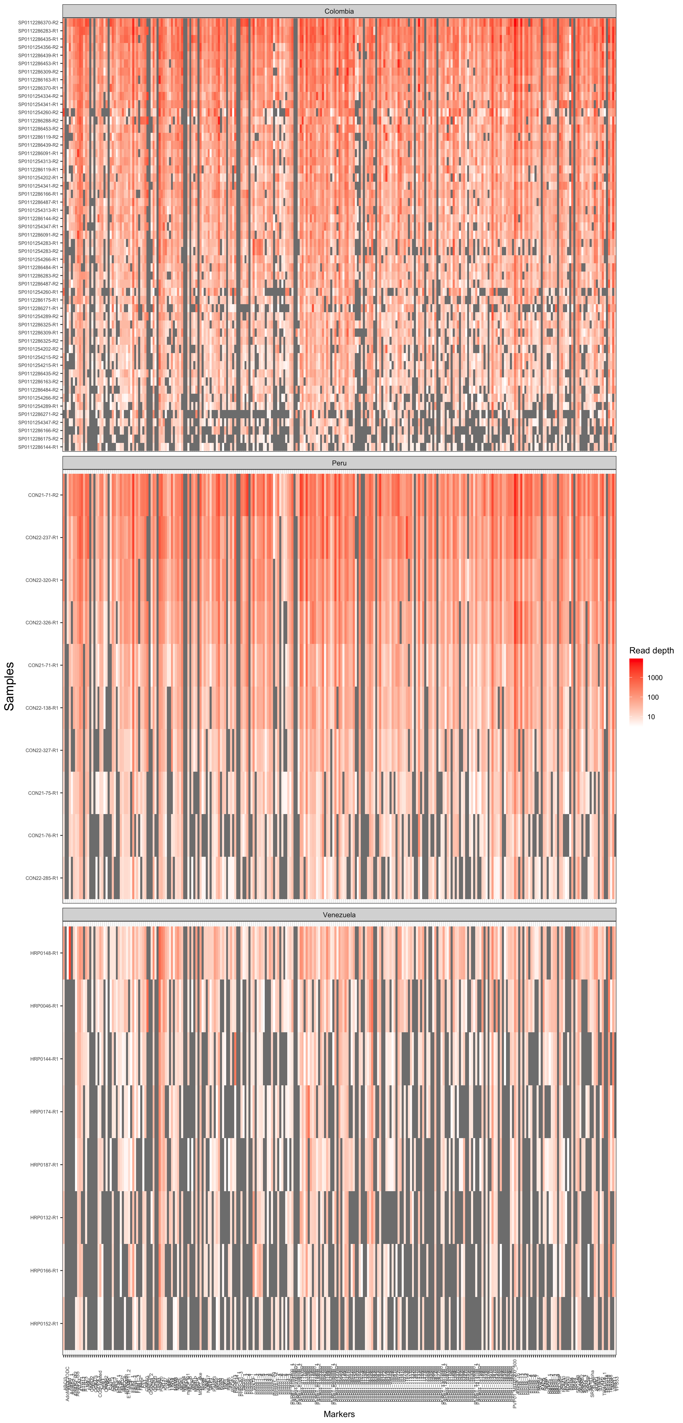
Figure 2: Read depth coverage of each samples and amplicon.
Then we can also use the function
loci_amplification_rate to measure the proportion of
samples that have been amplified by each amplicon marker.
ampseq_filtered = locus_amplification_rate(ampseq, threshold = .65, chr_lengths = c(
  1021664,
  956327,
  896704,
  1012024,
  1524814,
  1042791,
  1652210,
  1761288,
  2237066,
  1548844,
  2131221,
  3182763,
  2093556,
  3153402
))
Thus in this data set 271 loci had an amplification rate above 0.65,
and 58 loci were discarded. All discarded loci are stored in the slot
discarded_loci within the ampseq_object. The discarded loci
were: .
# Plot Amplification rate per loci ----
ggdraw()+
  draw_plot(ampseq_filtered@plots$amplification_rate_per_locus,
            x = 0,
            y = 0,
            width = 1,
            height = .5)+
  draw_plot(ampseq_filtered@plots$all_loci_amplification_rate,
            x = 0,
            y = .5,
            width = 1,
            height = .5)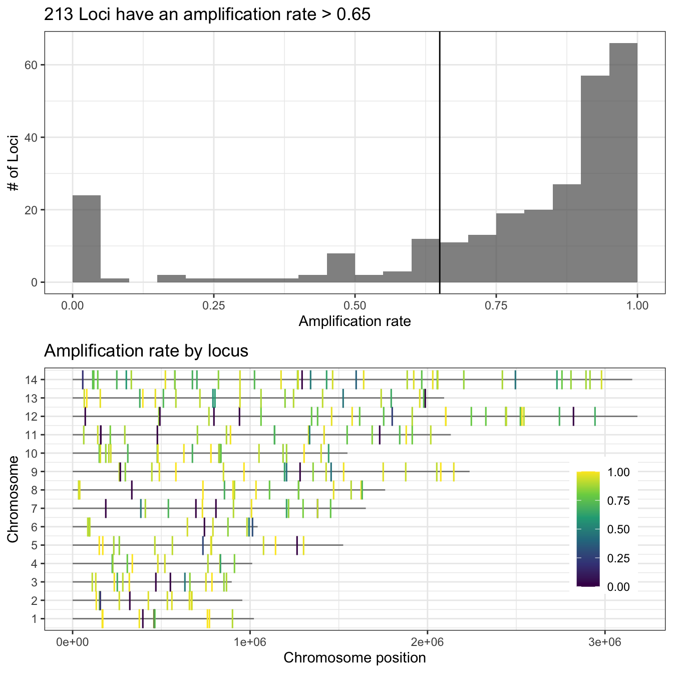
Figure 2: Proportion of amplified samples per locus. Top figure shows the distribution of the amplification rate (or proportion of amplified samples) of loci, with the number of loci in the y-axis and the amplification rate in the x-axis. Bottom figure shows the the chromosome location of each locus (chromosomes in y-axis and position in the x-axis) and the gradient color represents its amplification rate.
The next step is to measure the proportion of loci amplified per each sample, also called the amplification rate of the samples. For that purpose we are going to use the function sample_amplification_rate, and we are going to set the threshold equals to 0.6 (samples must amplify at least 60% of the total number of markers).
ampseq_filtered = sample_amplification_rate(ampseq_filtered, threshold = .6)

ampseq_filtered@plots$samples_amplification_rate+
         theme(axis.text = element_text(size = 12),
               axis.title = element_text(size = 12))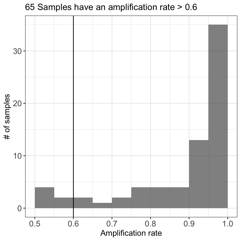
Figure 3: Proportion of amplified loci per sample. The figure shows the distribution of the amplification rate (or proportion of amplified loci) of the samples, with the number of samples in the y-axis and the amplification rate in the x-axis.
Molecular surveillance of drug resistance
Our panel of markers includes 10 genes (36 markers in total) that
could be associated with antimalarial resistance. In contrast to P.
falciparum where there is informartion about which polymorphims are
associated to resistance, in P. vivax that information is
missing. However, it is possible to report all observed polymorphism
respect to a reference sequence (in this case the strain Pv_P01). Just
as an example we are going to identify the aminoacid changes for the
genes mdr1, mrp1, and mrp2.
drug_resistant_haplotypes_plot = haplotypes_respect_to_reference(ampseq_object = ampseq_filtered,
                                        gene_names = c('pvmrp1',
                                                       'pvmrp2',
                                                       'pvmdr1'),
                                        gene_ids = c('PVP01_0203000',
                                                     'PVP01_1447300',
                                                     'PVP01_1010900'),
                                        gff_file = "docs/reference/Pviv_P01/genes.gff",
                                        fasta_file = "docs/reference/Pviv_P01/PvP01.v1.fasta",
                                        plo_haplo_freq = TRUE,
                                        variables = c('Sample_id', 'Population'),
                                        filters = NULL,
                                        na.var.rm = FALSE)


drug_resistant_haplotypes_plot$haplo_freq_plot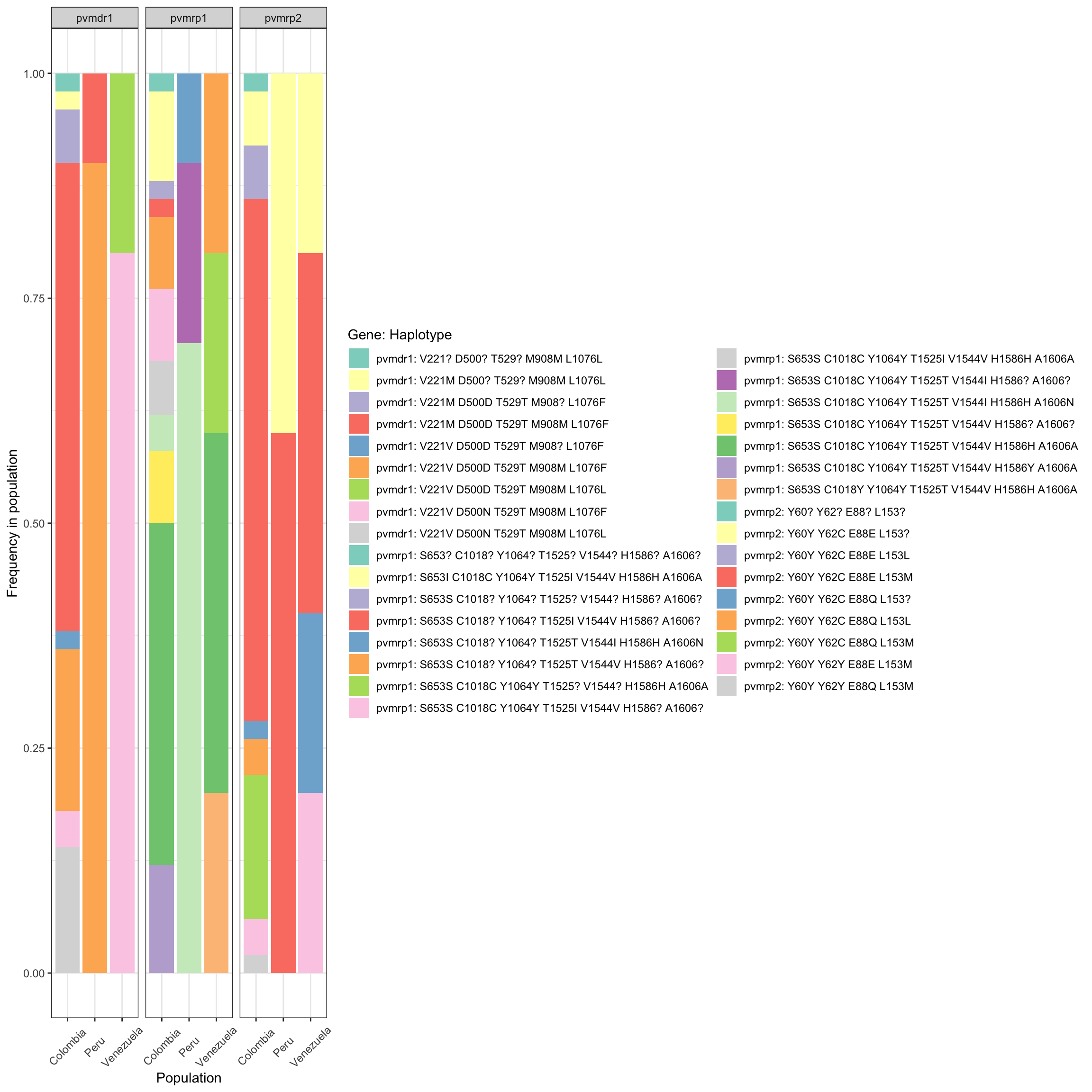
Population subdivision
The first step is to estimate the pairwise genetic relatedness using
the function pairwise_hmmIBD. As the dataset is small, we
won’t split the analysis in windows as we did for the
AMPLseq panel for P. falciparum.
# measuring relatedness----

if(!file.exists('docs/data/pvivax_pairwise_relatedness.csv')){
  pairwise_relatedness = pairwise_hmmIBD(ampseq_filtered, parallel = T)
  write.csv(pairwise_relatedness, 'docs/data/pvivax_pairwise_relatedness.csv', quote = F, row.names = F)
}else{
  pairwise_relatedness = read.csv('docs/data/pvivax_pairwise_relatedness.csv')
}
Now we can represent the relatedness network using the function
plot_network:
Relatedness_network = plot_network(pairwise_relatedness = pairwise_relatedness,
                               threshold = .90,
                               metadata = ampseq_filtered@metadata,
                               sample_id = 'Sample_id',
                               group_by = 'Population',
                               levels = c('Colombia', 'Peru', 'Venezuela'),
                               colors = c('firebrick3', 'dodgerblue3', 'gold3')
                              )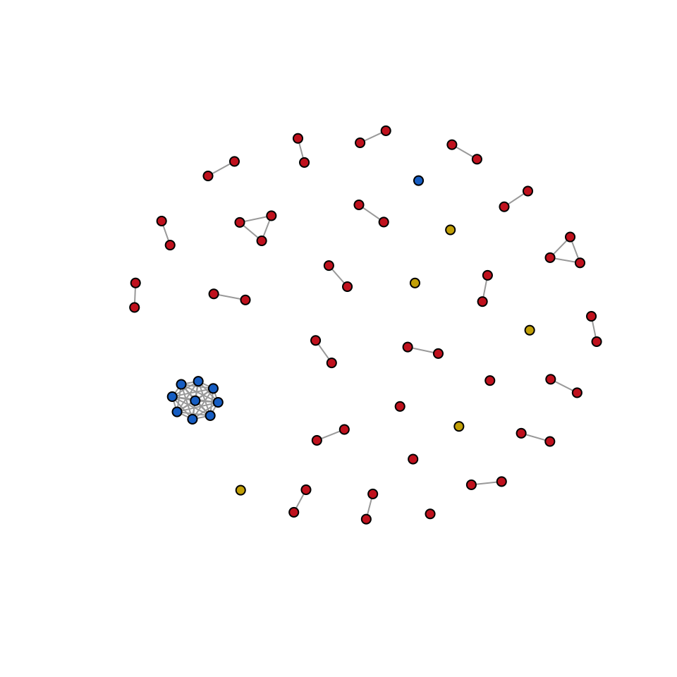
Figure 4: Network representation of pairwise genetic relatedness between samples. Each node represents a sample, and branches are displayed only for pairwise comparisons with a relatedness greater than 0.99. Colors were assigned based on the sampling location: Colombia (Red), Peru (Blue), and Venezuela (Gold).
Or, we can also observe the present of population structure using a PCA based on identity-by-descent (IBD).
evectors_IBD = IBD_evectors(ampseq_object = ampseq_filtered, relatedness_table = pairwise_relatedness, k = nrow(ampseq_filtered@metadata), Pop = 'Population', q = 2)


evectors_IBD %>% ggplot(aes(x = PC1, y = PC2, color = Population))+
  geom_point(alpha = .7, size = 2) +
  stat_ellipse(level = .6)+
  scale_color_manual(values = c('firebrick3', 'dodgerblue3', 'gold3'))+
  theme_bw()+
  labs(color = 'Countries')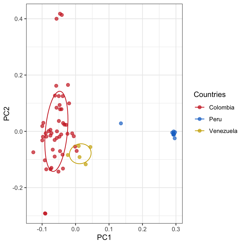
Figure 5: PCA of pairwise genetic relatedness between samples. Each node represents a sample, and colors were assigned based on the sampling location: Colombia (Red), Peru (Blue), and Venezuela (Gold).